Posted 07 July 2017
In my last post on this subject, I described a working 52Hz implementation of John Jenkins’ ‘degenerate N-Path Band-pass filter (BPF). This filter is intended to allow Wall-E2 (my wall-following robot) to discriminate between the IR homing beam from a charging station and other ambient IR interferers. This post describes the implementation of a basic swept-frequency square-wave function generator for use in testing BPF performance.
Now that I have a working (I think) version of the BPF algorithm, I want to implement and test a frequency and amplitude sweeping module so I can use it to test not only the working 52Hz BPF implementation, but the (so far not working) 520Hz implementation when we finally get the bugs worked out of it. My idea is that doing this now will have two (maybe three) significant benefits
- Allows me to fully characterize the existing 52Hz BPF implementation
- Gives me baseline performance characteristics for comparison against 520Hz results
- (freebie) – More fun with Teensy!
I’m already using a second Teensy 3.5 as the 52Hz square wave transmitter in my test setup, so all I need to do is to modify the existing program to sweep the desired frequencies and amplitudes. I think I’ll do this as a command-line parameter-entry program, with user-entry parameters for start, stop, and step frequencies (Hz) and fixed amplitude (% full-scale) for the frequency sweep module, and start, stop, and step amplitudes (% full-scale) and a set center freq for the amplitude sweep module.
12-15 July 2017 Update:
Well, I finally got the sweep generator going, at least the frequency sweep part, and managed to get some good data out of the 52Hz square wave demodulator. What I was striving for was something akin to the normal hardware setup where a frequency-sensitive ‘device under test’ (DUT) is driven from a frequency sweep generator, and a data logger of some sort records the result, something like the following block diagram. Back in the day, the ‘datalogger’ was quite often an engineer recording results on a piece of graph paper – how quaint! 😉
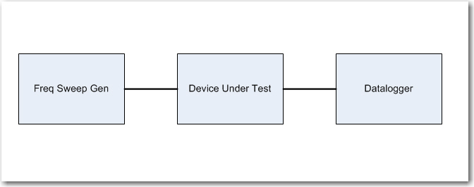
Typical swept frequency test setup
In this project, the DUT is the Teensy 3.5 hosting the IR demodulator code, and the frequency sweep generator is another Teensy 3.5 hosting the code to generate a swept-frequency square wave signal.
But, what to do about the datalogger? I could record data from inside the demodulator program, but we’re talking a lot of data; even at 52Hz that’s 52 4-byte values per second, and a sweep test might take as long as 3 minutes –> 36000 bytes. Fortunately, the Teensy 3.x sports 192KB of RAM, so a 36KB chunk barely scratches the paint – yay!! Another problem with logging internal to the demod module is how to correlate the captured data with the driving frequency; they are obviously correlated, but it’s not a slam-dunk to unequivocally assign particular frequencies to a particular stored data value.
So, I decided on a two-pronged approach; I will indeed save the data internally to RAM for later printout, but will also output an appropriately scaled version of the ‘final value’ calculation to one of the two DAC ports available on the Teensy 3.5 SBC. I plan to run this signal back to the sweep generator module so I can correlate ‘final value’ values with test frequencies, as shown in the following amended block diagram.
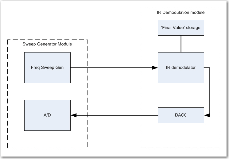
Modified sweep test block diagram
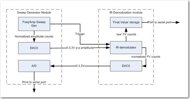
This setup works, and now I can get frequency-correlated ‘final value’ data from the sweep generator A/D. However, since the demodulator module ‘free-runs’ with respect to the sweep generator, the final value storage array can fill up before the frequency sweep finishes (or even before it starts!), so something is needed to synch the two modules. As the following block diagram shows, this is accomplished by providing a digital trigger from the sweep generator to start the demodulator. Also added in this final setup is the ability to set the square wave amplitude, for later amplitude sweep tests (set to 50% amplitude for the swept-frequency tests)
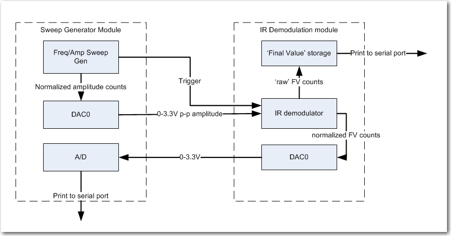
Final sweep setup. Note DAC block for square wave amplitude adjustment and trigger signal for synchronization
With the above setup I ran a number of frequency sweeps, as shown in the plots below. I started out with a sweep from 48 to 56Hz (+/- 4Hz from center freq), but quickly narrowed it down to +/- 2Hz. As my friend and mentor John Jenkins pointed out in his gentle, diplomatic way (something like “What were you thinking!“), the BPF bandwith is less than 1Hz, so a +/- 4Hz sweep range will just record a lot of nothing – oops!
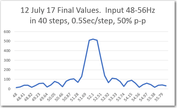
Frequency sweep results from sweep generator printout (D/A from IR demod, then A/D in sweep gen)
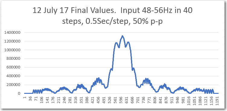
Captured ‘raw’ final value from IR demodulator. Frequency values added later
Even though the above sweeps were way too wide, it is clear that the demodulator algorithm is working (at least in the 52Hz implementation).
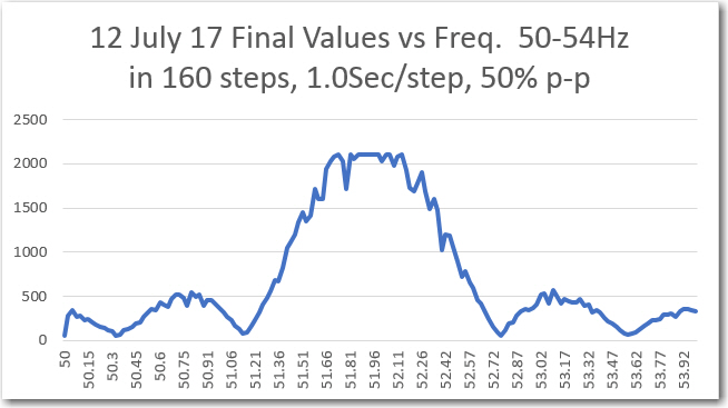
Frequency sweep results from sweep generator printout (D/A from IR demod, then A/D in sweep gen)
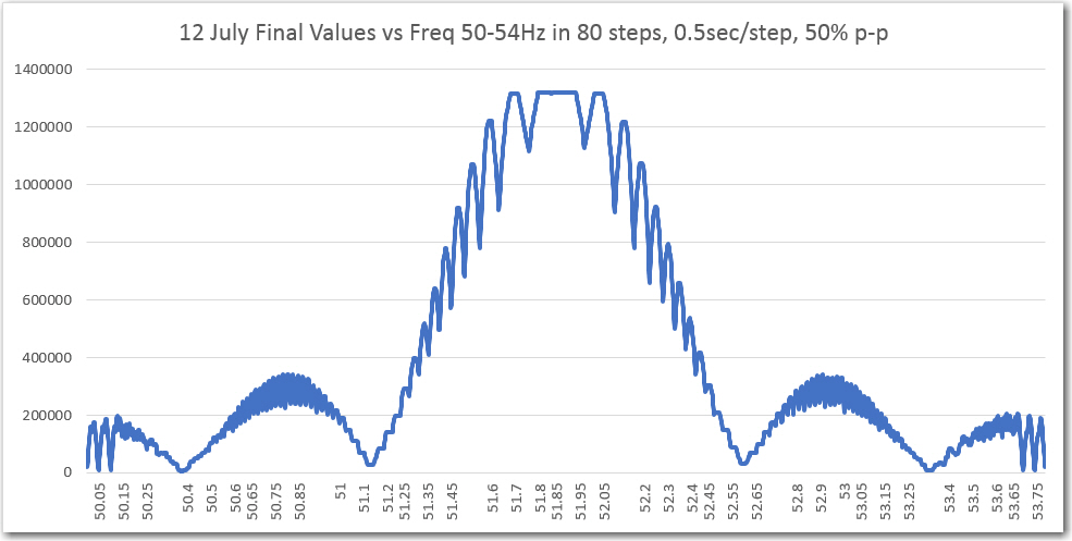
Captured ‘raw’ final value from IR demodulator. Frequency values added later
In the above plots, the sweep was reduced to +/- 2Hz, and the number of steps increased to 80. The result is a much more detailed look at the BPF response. As expected the general shape of the ’round-trip’ (individual ‘final value’ numbers sent from the demodulator to the sweep generator via the DAC-A/D channel and then printed) plot and the ‘raw final value’ plot match, but I didn’t expect either the flat-top region at the center of both plots or the fine ripple shown in the ‘raw’ plot. I made a number of additional sweeps with up to 160 steps at 2 sec/step, but neither the flat-top region nor the fine ripple features changed – they are apparently real features of the BPF response.
I think I finally figured out that the flat-top region was due to the fact that there is a narrow range of frequencies for which the filter response is maximum and identical. In this very narrow region, the digital sample points are ‘perfectly’ aligned with the incoming square wave, so that the final value is the maximum possible value for the input p-p amplitude.
As for the fine ripple features, I think these are due to the beat frequency between the incoming signal and the sample period. If this is the case, I would expect the ripple features to be more closely spaced far away from the center frequency, and less closely spaced toward the center. This certainly seems to be the case in the above plot, but even more evident in the detail plots below, (points extracted from the main plot above)
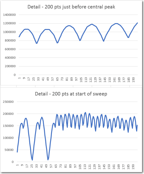
far and near center BPF response detail
Next, I performed an amplitude sweep from 100% to 0% p-p amplitude, with the center frequency set to 51.87Hz (this value was empirically determined earlier), with the following results
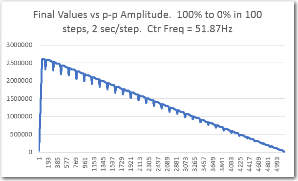
‘Raw’ final values from amplitude sweep.
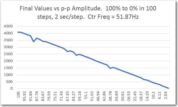
final values captured by sweep generator
As the above plots show, the filter response is very linear with respect to p-p amplitude variations. The maximum value shown in the ‘raw’ plot above is a little above 2.5 x 10⁶. The actual maximum value from the data is 2,606,752, which matches well with the theoretical maximum value of 4096*10*64 = 2,621,440.
Lastly, I performed another frequency sweep, but this time with a running-sum length of 32 cycles vs 64, to see how much the band-pass width was affected by halving the number of cycles in the running-sum circular buffer. Comparing the 32-cycle and 64-cycle plots as shown below, the ‘flat-top bandwidth is considerably wider than the original 64-cycle sweep results – about 1.8Hz edge-to-edge for 32 and about 0.4 for the original 64 version. Maybe as much as 4x bandwidth increase.
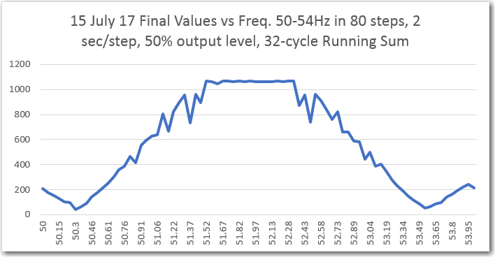
Frequency sweep results from sweep generator printout (D/A from IR demod, then A/D in sweep gen)
Frequency sweep results from sweep generator printout (D/A from IR demod, then A/D in sweep gen)
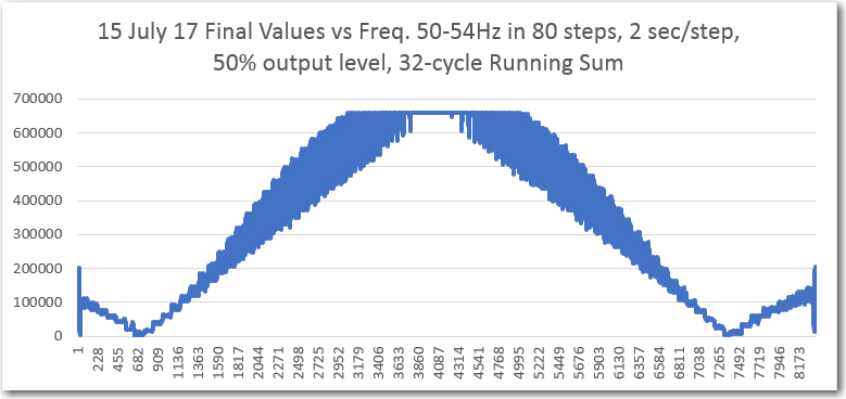
Captured ‘raw’ final value from IR demodulator.
Summary and Conclusions:
This post described my efforts to characterize the frequency and amplitude responses for the 52Hz implementation of the ‘degenerate N-path band-pass filter’ described to me by friend and mentor John Jenkins some time ago.
The original plan was to use this filter technique at 520Hz to enable my Wall-E2 wall-following robot to home to a charging station using a square-wave modulated IR signal to suppress ambient IR interference. Unfortunately, I could not get the 520Hz implementation to work properly, probably due to some unknown timing issues associated with the Teensy 3.x architecture. So, I decided to run the filter at 1/10th speed (52Hz) instead, thereby eliminating any timing issues, and allowing me to establish a baseline for subsequent higher-speed testing.
As the data above shows, the effort to implement the N-path BPF at 52Hz was completely successful. Both the frequency and amplitude responses were characterized. In addition:
- I gained a lot more experience with the Teensy 3.x line of SBCs. They are less than half the size of an Arduino Uno, have over 10x more RAM, 50x faster, come with on-board SD (3.5 & 3.6) cost about the same, and have about the same power requirements – such a deal!
- Implemented a Teensy 3.5 frequency/amplitude sweep square wave generator, and verified proper operation by using it to characterize the 52Hz BPF implementation.
- Implemented a Teensy 3.5 fixed-frequency square wave generator, and verified proper operation by using it to find the correct transmit frequency for the 52Hz BPF implementation
- Validated the efficacy of my little two-Teensy test bed.
The above tools can now be used with high confidence to investigate (and hopefully eliminate) the problems with running the BPF at 520Hz.
Stay tuned!
Frank
Pingback: IR Modulation Processing Algorithm Development – Part XV - Paynter's Palace