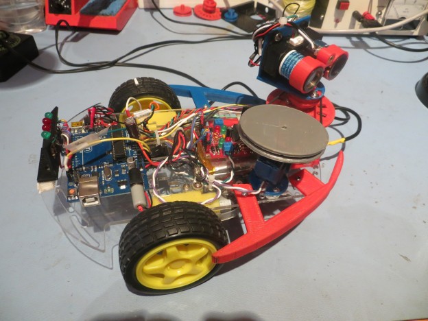
Back in May of this year  I purchased a 4-wheel drive robot kit from DFRobots as a possible successor to my then-current Wall-E 3-wheel (2 drive motors and a small castering nose wheel). I didn’t have time to do more than just assemble the basic kit (see this post), so it spent the intervening months gathering dust on my shelf.  Coincidentally, my wife arranged with our  son to kidnap her grand-kids for a week (giving our son and his wife a much-needed break, and giving us some quality grand-kid time), so I decided to brush off the 4WD robot kit as a fun project to do with them, in parallel with re-working Wall-E to remove its spinning LIDAR assembly and replace it with a hybrid LIDAR/Sonar setup.

The plan with the 4WD robot is to incorporate another spinning-LIDAR setup – this one utilizing the XV-11 spinning LIDAR system from the NEATO vacuum cleaner.  This system rotates at approximately 300 RPM (5 RPS), so there is a decent chance that will be fast enough for effective wall navigation (the Wall-E LIDAR setup couldn’t manage more than about 200 RPM and that just wasn’t good enough).

However, before we get to the point of determining whether or not the XV-11 LIDAR system will work, there is a LOT of work to be done.  At the moment, I can see that there are four major subsystems to be implemented

• Battery Supply and Charger
• Motor Controller integration
• XV-11 LIDAR controller
• Navigation controller

Battery Supply and Charger

In preparation for the project, I purchased 2ea 2000 mAH Li-Ion batteries and a supply of ‘basic Li-Ion charger’ modules from SparkFun.  In my previous work with Wall-E, I had devised a pretty decent scheme for charge/run switching using a small 2-pole, double-throw relay to switch the battery pack from series connection for running the robot to independent-parallel for charging, so I planned to use the same setup here.  After the usual number of screwups, I wound up with a modular battery pack system that could be tucked away in the motor compartment of the 4WD robot.

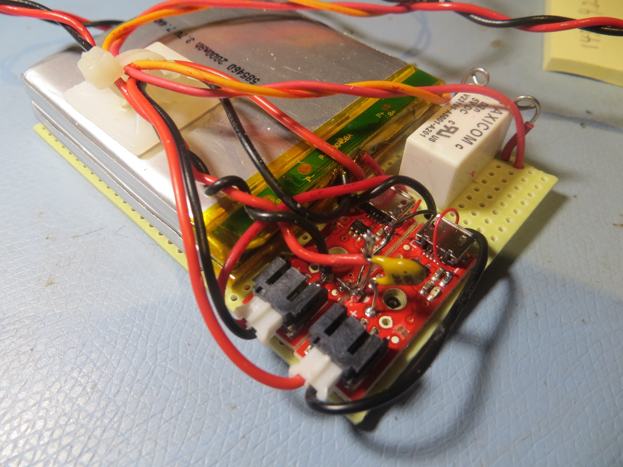
Battery pack showing charging modules and switching relay. The tan capacitor-looking component is actually a re-settable fuse

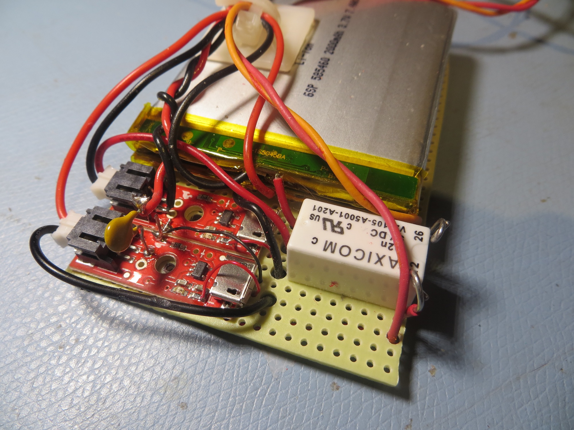
Battery pack showing charging modules and switching relay. The tan capacitor-looking component is actually a re-settable fuse

In the above photos, the tan component that looks very much like a non-polarized capacitor is actually a re-settable fuse!  I really did not want to tuck this battery pack away in a relatively inaccessible location without some way of preventing a short-circuit from causing a fire or worse.  After some quality time with Google on the inet, I found a Wikipedia entry for ‘polymeric positive temperature coefficient device (PPTC, commonly known as a resettable fuse, polyfuse or polyswitch).  These devices transition from a low to a high resistance state when they get hot enough – i.e. when the current through them stays above a threshold level for long enough.  They aren’t fast (switching time on the order of seconds for 5X current overload conditions), but speed isn’t really a factor for this application.  I don’t really care if I lose a controller board or two, as long as I don’t burn the house down.  Even better, these devices reset some  time after the overload condition disappears, so (assuming the batteries themselves weren’t toasted by the overload), recovery might be as simple as ‘don’t do that!’.

Motor Controller Integration

When I got the 4WD robot kit, I also purchased the DFRobots ‘Romeo’ controller module. This module integrates an Arduino Uno-like device with dual H-bridge motor controllers with outputs for all 4 drive motors.  Unfortunately, the Romeo controller has only one hardware serial port, and I need two for this project (one for the PC connection, and one to receive data from the XV-11 LIDAR).  So, I plan to use two Solarbotics dual-motor controllers, and an Arduino Mega as the controller

XV-11 LIDAR Controller

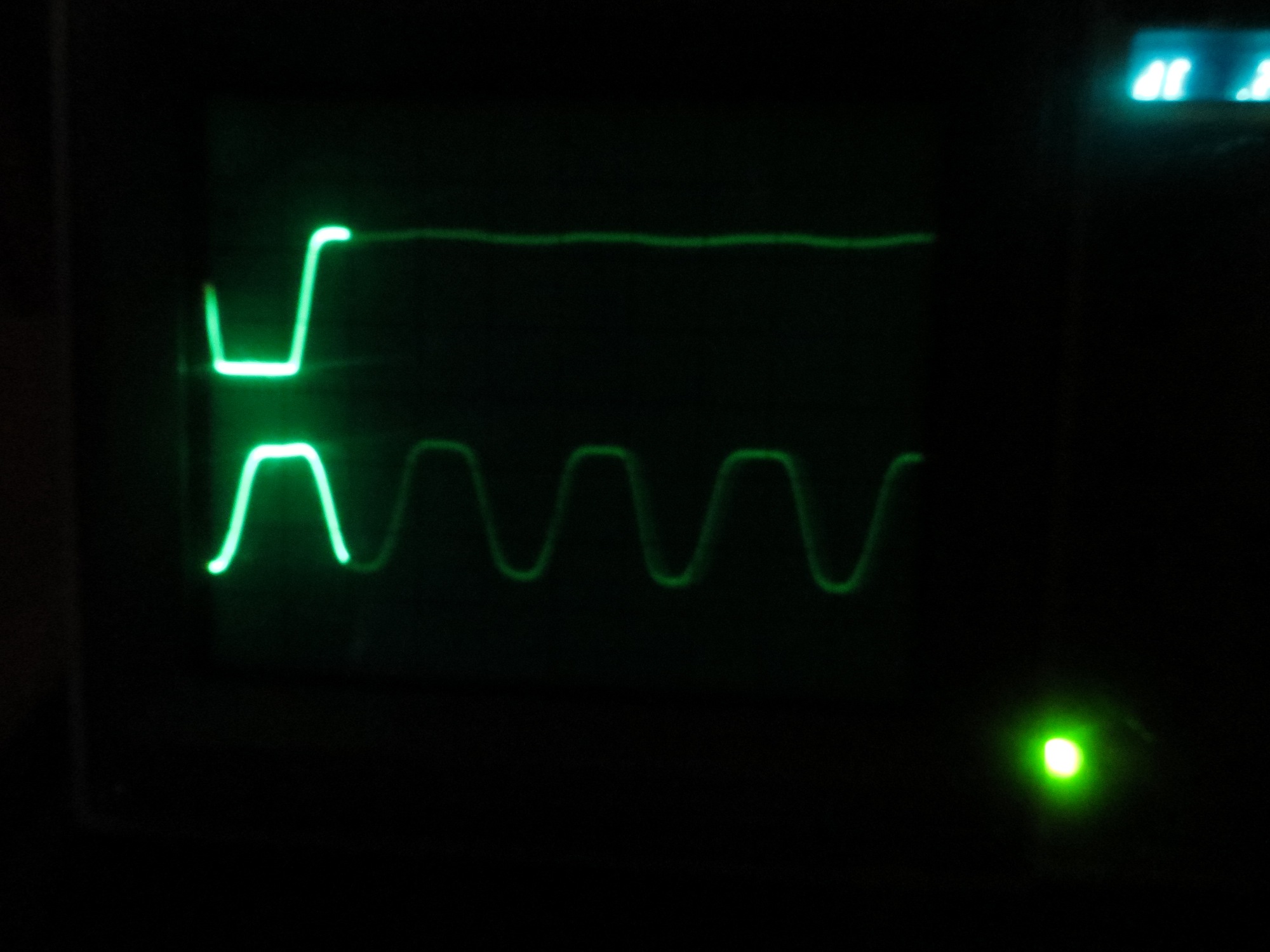
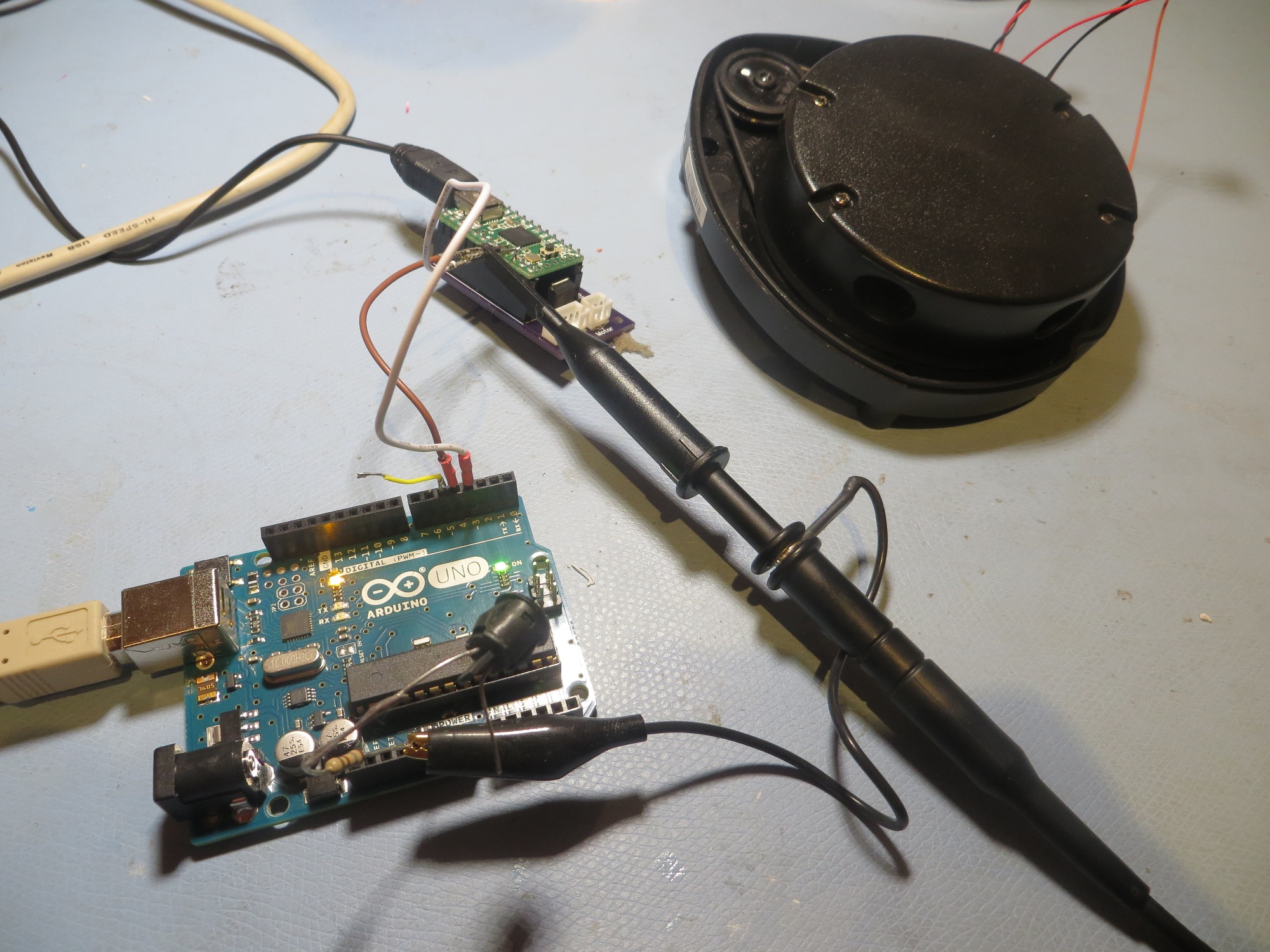
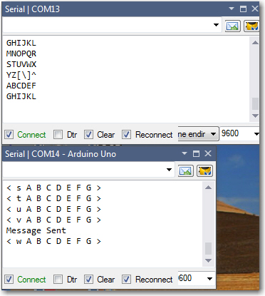
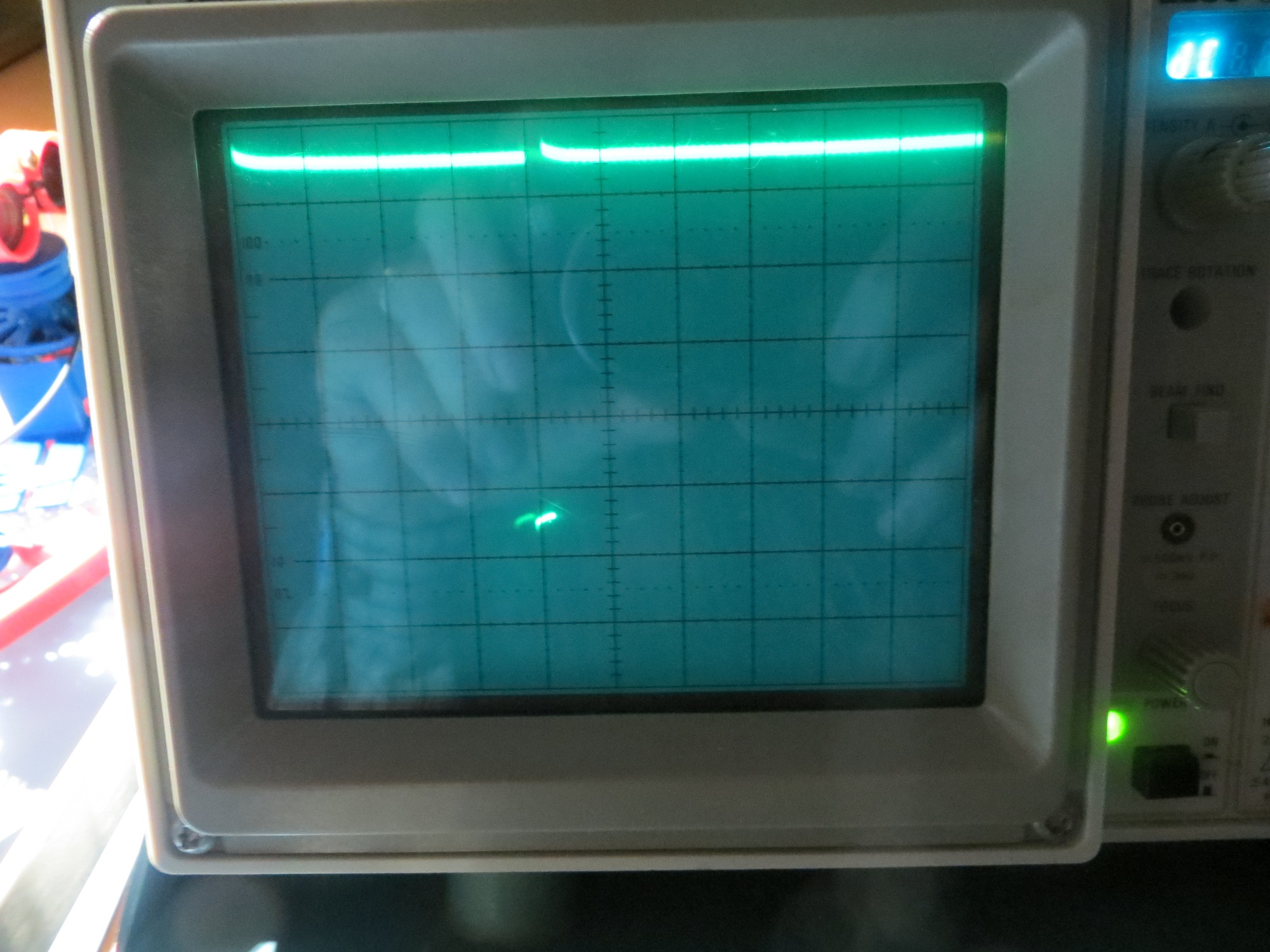
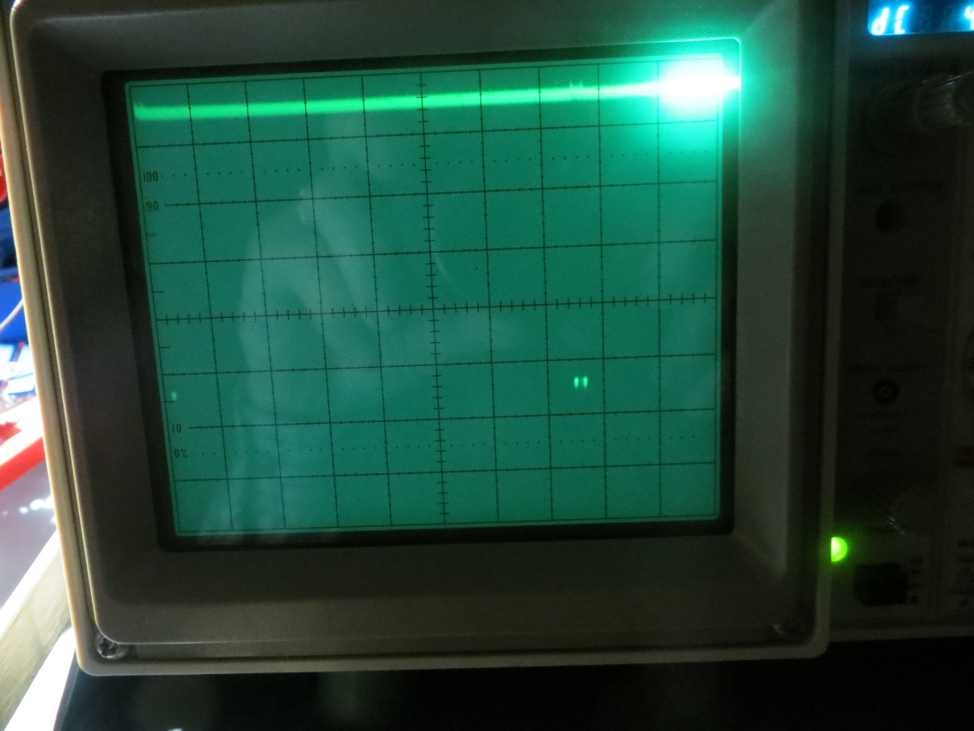
The XV-11 LIDAR from the NEATO vacuum has two interfaces; a 2-wire motor drive that expects a  PID signal from a FET driver, and a high-speed serial output that transfers packets containing  RPM, status, and distance  data.  A company called ‘Get Surreal’ has a really nice Teensy2.0-based module and demo software that takes all the guesswork out of controlling the XV-11, but its only output is to a serial monitor window on a PC.  Somehow I have to get the data from the XV-11, decode it to extract RPM and distance data, and use the information for navigation.  The answer I came up with was to use the Get Surreal PCB without the Teensy as sort of a ‘dongle’ to allow me to control the XV-11 from an Arduino Mega.  XV-11 serial data is re-routed from the Teensy PCB connector to Rx1 on the Arduino Mega.  The Mega, running  the same demo code as the Teensy, decodes the serial packets, extracts the RPM data and provides the required PID signal back to the driver FET on the Teensy PCB.  Not particularly fancy, but it works!

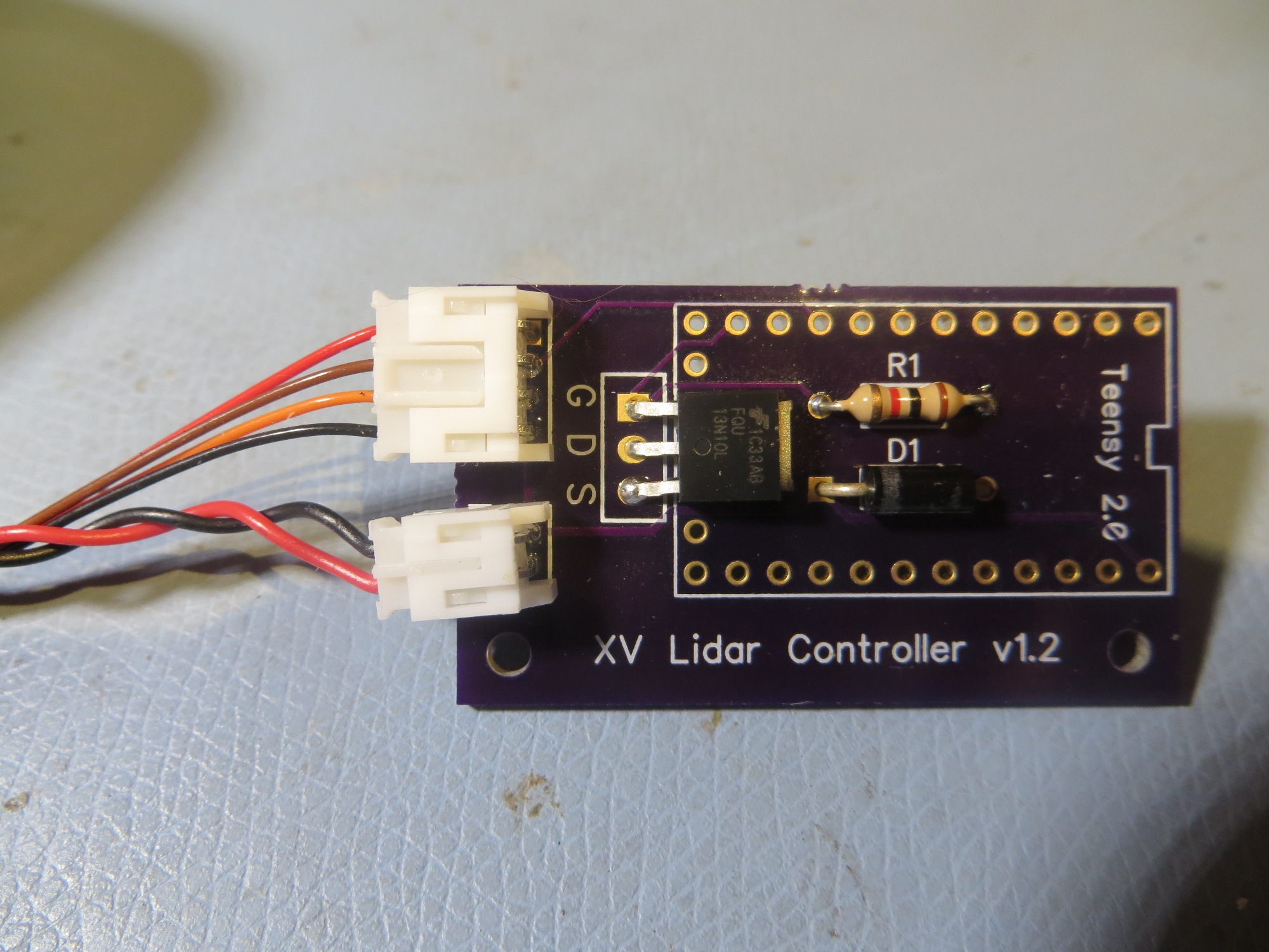
XV-11 Controller V1.1 without the Teensy 2. The original connectors were replaced with right-angle versions

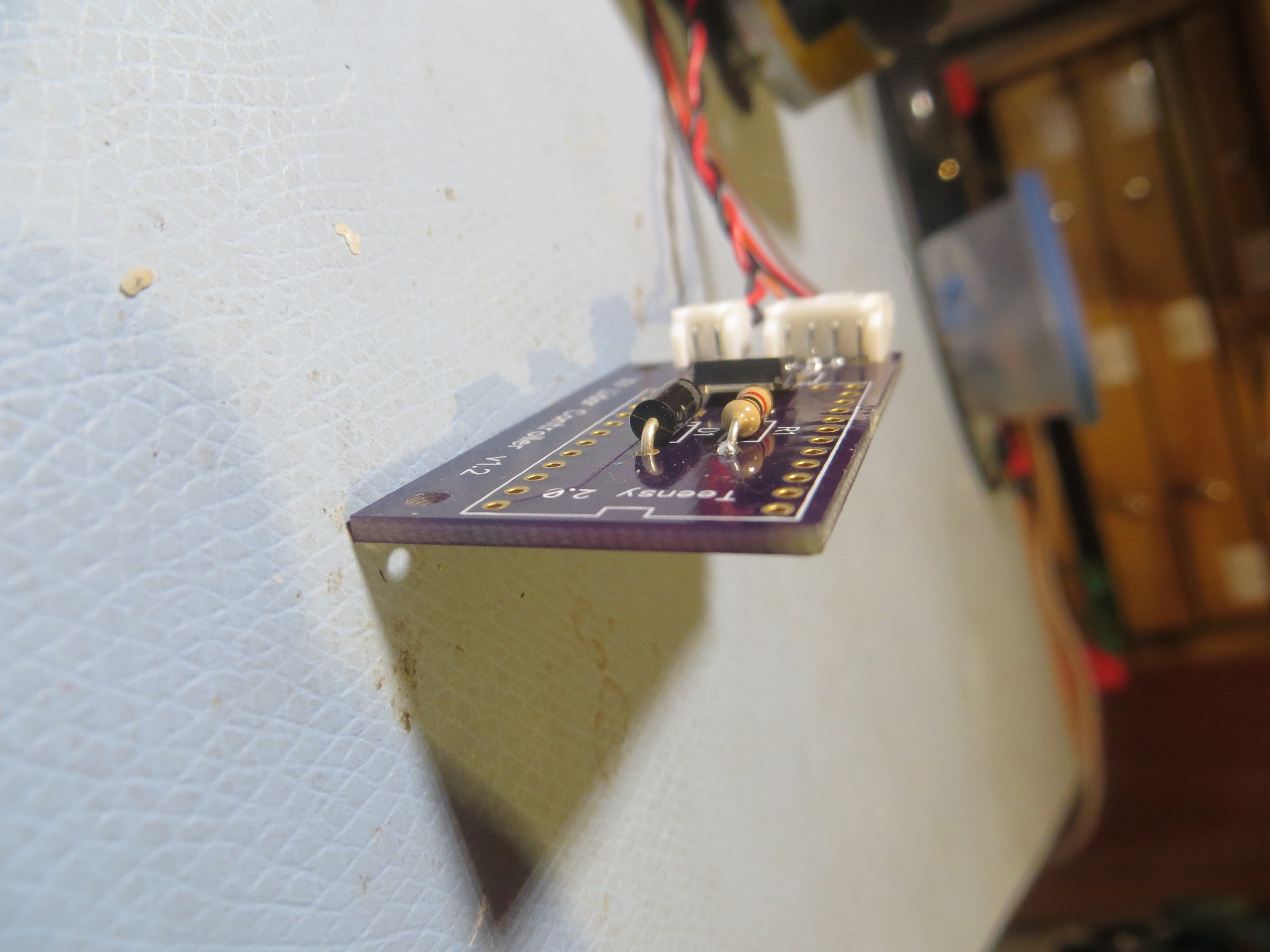
Side view of the XV-11. The right-angle connectors lower the height considerably

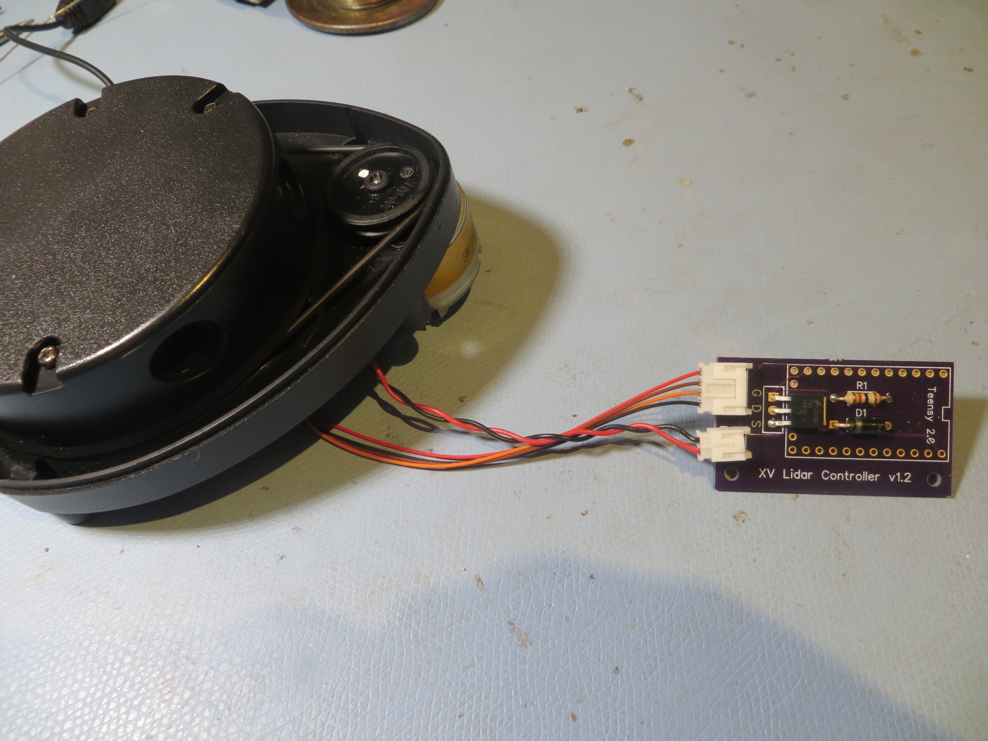
XV-11 connected to the ‘controller dongle’

The ‘before’ and ‘after’ versions of the XV-11 controller

During testing of the ‘XV-11 dongle’, I discovered an unintended consequence of the change from upright to right-angle connectors.  As it turned out, the right-angle connectors caused the pin assignments to be reversed – yikes!  My initial reaction to this was to simply pull the pins from the XV-11 connectors and re-insert them into the now-proper places.  Unfortunately, this meant that I could no longer go back to controlling the XV-11 from the original controller module – bummer.  So, I wound up constructing two short converter cables to convert the now-reversed XV-11 cables to the ‘normal’ sense for the Get Surreal controller module.  Nothing is ever simple….

Navigation Controller

The navigation controller for the 4WD robot will be an Arduino MEGA 2560.  This board was chosen because it has LOTS of digital/analog/pwm I/O and multiple hardware serial ports.  You can’t have too many I/O ports, and I need at least two (one for the USB connection the host PC, and one to interface to the NEATO XV-11 spinning LIDAR) hardware serial ports.  The downside to using the Mega is its size – almost twice the area of the Arduino Uno.

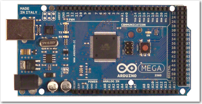
Arduino Mega 2560 for LIDAR I/O and navigation control

30 September, 2015

Sad to say, but I believe I have ‘hit the wall’ on development of an effective spinning-LIDAR navigation system for Wall-E.  Even with a souped-up spinning platform (approx 3 rev/sec), I have been unable to reliably navigate a straight hallway, much less recover from stuck conditions.  In addition, the combination of drive motor currents and the increased current required to drive the spinning platform at the increased rate drains  the battery in just a few minutes.  So, I have reluctantly concluded that the idea of completely replacing the acoustic sensors with a spinning-LIDAR system is a dead end; I’m going to have to go back to the original idea of using the acoustic sensors for wall following, and a fixed-orientation LIDAR for stuck detection/recovery.

I started down the spinning-LIDAR road back in April of this year, after concluding a series of tests  that proved (at least to me) that the use of multiple acoustic sensors was not going to work due to intractable multi-path and self-interference problems.  In a follow-up post at the end of that month, I speculated that I might be able to replace all the acoustic sensors  with  a spinning-LIDAR system for both wall following and ‘stuck detection’.  At the time I was aware of two good candidates for such a system – the NEATO XV-11 robot vacuum’s spinning-LIDAR subsystem, and the Pulsed Light ‘LIDAR-Lite’ component.  I chose to pursue the Pulsed-Light option because it was much smaller and lighter than the XV-11 module, and I thought it would be easier to integrate onto the existing Wall-E platform.  Part of the appeal of this option was the desire to see if I could design and build the necessary spinning platform for the LIDAR-Lite device, based on a 6-wire slipring component available through AdaFruit.

In the time since that post at the end of April, I successfully integrated the LIDAR into the Wall-E platform, but only recently got to the point of doing field tests.  The first set of tests showed me that the original spin rate of about 120 RPM (about 2 RPS) was way too slow for successful wall following using my original ‘differential min-distance’ technique, and so I spent some time investigating PID control techniques as a possibility to improve navigation.  Unfortunately, this too proved unfruitful, so I then investigated ideas for increasing the LIDAR’s spin rate.  The LIDAR spinning platform is driven by a drive belt (rubber O-ring) attached to a pulley on a separate 120 RPM DC motor.  My original setup used a pulley ratio of approximately 1:1, so the motor and LIDAR both rotated at approximately 120 RPM.  By increasing the diameter of the drive pulley, I was able to increase the LIDAR rotation rate to approximately 180 RPM (about 3 RPS), but unfortunately even that rate was too slow, and the increased drive motor current rapidly drained the batteries – rats!

‘The Last Spinning LIDAR’ version. Note the large gray drive pulley. Gets the spin rate up to around 180 RPM, but at the cost of much higher battery drain.

So, while I had a LOT of fun, and learned a lot in the process, it’s time to say ‘Sayonara’ to the spinning-LIDAR concept (at least for Wall-E – still plan to try the XV-11 module on the 4WD robot) and go back to the idea of using acoustic sensors for wall following and a forward-looking LIDAR for obstacle avoidance and ‘stuck’ detection.

Stay tuned!

Posted 17 September, 2015

After getting the improved tachometer assembly  integrated into Wall-E’s spinning LIDAR setup, I decided to repeat the hallway  field testing that I performed back in July of this year (see this post for the details).  My ‘theory of navigation’ for wall following is that I should be able to determine Wall-E’s orientation relative to a nearby wall by looking at where the spinning LIDAR’s minimum distance measurement occurs relative to Wall-E’s ‘nose’.

Just as I did back in July, I placed  Wall-E a short distance away from a long straight wall, in three different orientations – parallel, 45-deg nose-in, and 45-deg nose-out.  For each of these orientations I let the spinning LIDAR ‘look’ at the wall for about 10 revolutions, and then I manually changed the orientation. The distance and angle (actually the interrupt number, but that is the same as the angle) values were recorded in a text log.

The LIDAR Field Test Area. Note the dreaded fuzzy slippers are still lurking in the background

Wall-E oriented at approximately 45 degrees nose-out

Wall-E oriented at approximately 45 degrees nose-in

Wall-E in the ‘parallel’ configuration

LIDAR distance measurements to a nearby long wall

The text log was arranged as shown in the following screenshot.

A small portion of the data log for the wall orientation test. Note the line at the top describing the orientation sequence

Next, I wrote an Excel VBA script to parse the text log file and extract just the half of each revolution where the LIDAR was scanning the nearby wall, skipping over the half.  For each such scan, I searched the distance data for the minimum value, capturing that value and its associated interrupt number (i.e. angle).  All the extracted distance values and the min dist/min angle numbers were written to the spreadsheet, and then I plotted the mininum distance interrupt  number (i.e. angle) vs rev number for about 90 LIDAR revolutions.

If my theory holds water, then I should be able to see variations in the minimum interrupt number over time that corresponds to the orientation changes.  As shown in the following plot, that is exactly what happens.

Excel plot of the interrupt number corresponding to minimum distance vs rev number

As can be seen in the above plot, the Min-Dist-interrupt (MDI) starts out between 4 and 5, and stays there for the first 9-10 revolutions.  At about rev 11, it jumps to the 7-8 range, where it stays until about rev 20. The it drops back to 5-6 for 10 revs, and then drops again to the 2-3 range.  This pattern then repeats for the duration of the plot.  In my current spinning LIDAR configuration, Interrupt 1 starts at Wall-E’s tail, and proceeds along Wall-E’s left side to interrupt 10 at the nose.  So, an MDI of 4-5 should correspond to the parallel orientation, while a lower number should correspond to nose-out and a higher one to nose-in.  From the test condition description, Wall-E was placed parallel for 10 revs, then nose-in for 10, then nose-out for 10, then back to parallel, repeat.    It is clear from the plot that the actual behavior of the MDI matches the predicted behavior quite nicely – EUREKA!! ;-).

Although the above test results are quite encouraging, it is still not entirely clear that this technique can actually be used for effective navigation at practical travel speeds.  There is undoubtedly some correlation between the spinning LIDAR rotation rate and the maximum travel speed at which the LIDAR can provide information fast enough for effective steering.  For instance, the NEATO XV-11 spinning LIDAR system rotates at about 300 RPM (5 RPS), and it seems to travel no faster than about 1-2 m/sec.  This might mean that my 120 RPM (2 RPS) spin rate would only support travel speeds in the 0.5-1 m/sec range.  In addition, my current 18-degree resolution may be too coarse for effective steering.  Again using the XV-11 as a baseline, it has a resolution of 1 degree, 18 times mine.  With the much faster speed of the new V2 ‘Blue Label’ Pulsed Light LIDAR, I could probably double or even triple my current angular resolution, but 18X might be a bit much ;-).

Next up – analyzing the data from a simulated navigation test, where I manually pushed Wall-E along the hallway, simulating as close as possible how I think Wall-E might navigate, assuming the spinning LIDAR data is fast enough and accurate enough.  As I moved Wall-E along, I recorded the same distance and interrupt number data as before, so it will be interesting to see if this data continues to support my current ‘theory of navigation’ – stay tuned!

22 September 2015 Update:   The data from the simulated navigation test was a mess – nothing recognizable as a pattern.  The one thing it  did do was convince me that the ‘angle of least distance’ idea wasn’t going to work – and that something else was going to have to be done. What, I don’t know  yet…

Frank

Posted 16 September, 2015

Back in June of this year I posted about my initial efforts to implement a tachometer subsystem as part of a spinning-LIDAR system (see ‘LIDAR-Lite Gets its Own Motor‘),  This implementation used a ‘plugged gap’ technique for detecting the index position of the LIDAR, as shown below.

Diagram of the tach wheel for Wall-E’s spinning LIDAR system

The idea was that when the time between gap interrupts was more than 2 gap durations (assuming a relatively constant rotation speed), then the ‘plugged gap’ must be between the IR LED and the photo-diode.  This design  works OK, but has a couple of nagging drawbacks:

• It depends on a fixed  open-loop timing delay; if the motor RPM varies enough, the fixed delay threshold might be too large or too small.
• The plugged-gap technique removes two interrupt positions from the wheel, meaning that position information is missing during that 54-degree arc.

So, after getting my V2 ‘Blue Label’ LIDAR from Pulsed Light and figuring out how to use it (see this post), I decided to see what I could do about addressing  both the above problems.  At first I  thought I might be able to simply add a second photo-diode on the sensor side of the tach sensor assembly, coupled to the existing single IR LED via a slanted channel in the tach wheel, as shown below.  The idea was that when the interrupt was fired at the edge of the index gap, the value of the  ‘other’ sensor could be read – if the value was below a certain threshold (meaning more impinging IR energy), then that sensor must be lined up with  the index hole.  This meant that the index hole needed to be offset from the index gap, so the max energy receive position would coincide with the position at which the interrupt fired, which occurs at the gap edges,  not the center.

This turned out to be a miserable failure.  The IR LED’s have a very narrow illumination sector, and there wasn’t enough off-axis energy to reliably detect the index hole.

So, some five versions later, along with a complete redesign of the sensor assembly, I have what I think is a nicely working implementation.  The single LED slanted-hole design was scrapped in favor of a two-LED/sensor one, and the index sensing hole was replaced by a circumferential gap, as shown below.

Latest two-sensor/LED design. Note the circumferential gap is centered on one edge of the index gap, so the index sensor voltage will be minimum (max incident energy) when the gap-edge interrupt fires.

For the tach sensor assembly, the single IR LED was replaced by two independent IR LED’s, each with its own 240-ohm current-limiting resistor (I tried running them in series with a single resistor, but that didn’t work very well either).  The original enclosed sensor slot was replaced by an exposed ‘trough’ with two retainer bars (the trough without the retainer bars didn’t work either).  See below for the ‘new improved’ tach sensor assembly.

Tach sensor assembly showing the mounting holes for the two 3mm IR LED’s . The thin gaps visible in the background are the corresponding channels into the photo-diode trough

Tach sensor assembly showing the photo-diode trough. The backs of the photo-diodes are glued to a thin plastic carrier that is captured by the retaining bars

After running some preliminary tests, I mounted  the new tach wheel and sensor assemblies and ran some O’scope tests to see how the new design worked.  I was  very pleased to see that it appears  to be working better than I could have hoped.  In the following O’scope photo, the top trace is the index sensor, and the bottom trace is the normal tach-gap sensor.  Both are 2 volts/cm and exhibit full 5-volt swings.

O’so;pe photo with the signal of interest highlighted. The top trace is the index sensor, and the bottom one is the tach-gap sensor.  The index interrupt will occur at the first rising edge of the bottom trace.

The gap interrupt of interest occurs at the first rising edge of the bottom trace.  As can be seen from the photo, reading the value for the index gap sensor (top trace) at this point will retrieve a stable ‘0’ value, perfect for index gap detection!

The following photos show the new tach wheel and sensor assembly mounted on Wall-E, with the LIDAR assembly removed for clarity.

Stay tuned for more test results from this configuration!

Posted 17 September, 2015:

After re-installing the LIDAR and making all the right connections (not a trivial task, btw), I fired the system up using my ‘DAFAP_Plus’ (that’s. “Distance as Fast as Possible’ plus modifications for interrupt handling) sketch and took some index sensor measurements.  In the screenshot below, the ‘Sensor’ values are from the index sensor.  As expected, they are near the top of the 10-bit A/D range for interrupt numbers 1-19 (a reading of 700 implies about 3.5VDC).  However, the sensor reading for interrupt 20 is now  much better than it was before; before implementing the improved LED driver and new tach wheel layout, the max readings were about the same, but the minimum reading was occasionally  over 400 (i.e. about 2VDC) – making it harder to reliably discriminate between non-index and index gap  cases.  Now the index gap reading is a reliable ‘0’, providing a 3.5VDC differential – more than double the 1.5VDC  differential before – yay!!

Another item of note in the readout below is the ISR Ms value.  This is the time required to service the associated interrupt,  including the time required for the Pulsed Light ‘Blue Label’ LIDAR to take a distance measurement. Note that all of these times are in the single digit range – meaning I could probably double the number of tach wheel gaps (i.e. double the system angular resolution) if I wanted to.  Note that there is an extra value shown for each ‘interrupt 20’ line; this ‘Idx Ms’ value is the total time between index gap appearances, i.e. the total rotation time.  So, the LIDAR is rotating just a tad shy of 120 RPM (2 RPS), which should be fast enough for decent wall-following navigation.

Log from a 17 Sept 2015 test run; note the ‘0’ sensor value at interrupt 20

Frank

Posted 08/24/2015

Progress on the Pulsed Light ‘Blue Label’ spinning LIDAR system has been put on hold for a few days pending the arrival of some 3mm IR LEDs  needed for an upgraded tach sensor wheel, so I am passing the time working on the alternative system, the XV-11 LIDAR module from the NEATO vacuum.

Back in May of this year I posted some results where I mated the Teensy 2.0 based Get Sureal XV-11 module controller (see the post here) and got very good results with a LIDAR ‘image’ of the walls of a cardboard box.  After this effort, I put the XV-11 aside for two reasons; first, I received a ‘Silver Label’ (V1) LIDAR-Lite unit from Pulsed Light and was having too much fun designing and implementing a spinning-LIDAR system, and second, I couldn’t figure out how to get the XV-11 data into my robot controller (an Arduino Uno).  The Teensy 2.0 XV-11 controller parses the data stream from the XV-11, routes it upstream to the USB host, processes commands from the USB host, and maintains the XV-11 rotation speed using a PID controller.  This is all well and good, but the Uno isn’t a USB host, and adding that capability would be a major PITA.  So, I put the whole thing on the back burner, hoping that inspiration would strike at some later date.

Now, almost three months later, I had some ideas I wanted to try to achieve the  goal of getting the XV-11 streaming data onto the Uno robot controller so that it could be used for navigation.

The Problem(s):

The XV-11 LIDAR module streams angle, position, data-quality, and RPM information over a serial connection to the Teensy 2.0 controller, and there is a LOT of it.  The XV-11 rotates at a nominal rate of 300 RPM, i.e. 5 RPS.  During every 200 msec rotation, it sends 360 (at least) data groups, where each data group contains pointing angle (0-360), distance (in cm, I think), a data quality metric, and RPM.  Each data group must be parsed to extract the needed information.  The Teensy firmware also provides a PWM waveform to control the XV-11’s rotation speed, based on the RPM values being reported over the serial port.

The Teensy 2.0 boasts two hardware serial ports, but one is used for the connection to the upstream USB host,  and the other one is used to receive the data from the XV-11.  So, no easy way to get the needed XV-11 data from the Teensy to the Uno – bummer :-(.  And, even if the Teensy had a third hardware serial port, the Uno only has one – and it is used to connect to its upstream USB host – double bummer :-(.

And, even if I could figure out a way to get the data over to the Uno, how was I going to keep the data stream from  swamping the Uno’s (or the Teensy’s) very finite resources.  With the spinning LIDAR system,  I only capture 18 data groups/revolution, and even this amount threatens to blow out the top of working memory.  There is no way it can handle the 360 data groups from the XV-11.  Moreover, those data groups are arriving at about twice the rate of the groups from the Pulsed Light spinning LIDAR system.

The (partial) Solution – Software Serial to the Rescue!:

In between times where I was actively working on the Pulsed Light spinning LIDAR project, I kept returning to the problem of how to get XV-11 data into the Uno, and in my wanderings through the online Arduino world I ran across references to ‘Software Serial’, where virtual serial ports could be implemented using two of the Arduino GPIO pins.  This sounded intriguing, but all the available libraries come with baggage of one sort or another; one can’t send/receive simultaneously, another can do that, but is sensitive to other interrupts…  Then, just the other day I ran across ‘SimpleSoftSerial’ a version written by ‘Robin2’ just for the Uno (see the post here).  The whole thing is just a ‘.ino’ file, not a library at all, and it does exactly what I want – YAY!  Having the ability to add another serial port to the Uno solves part of the problem, so I decided to see if I could get just this part going, and maybe figure out the data management issue at some future time.

Robin2 also kindly provided a pair of Arduino sketches to demo the ‘Simple SoftSerial’ capability. One part runs on a Uno (of course, as that is the target processor for this little hack) and the other ‘Partner’ program runs on (in his case) a Mega as it requires multiple hardware  serial ports.  I didn’t have a Mega handy, but I  did have the Teensy 2.0 that came with the Get Sureal XV-11 controller, and it has two hardware serial ports.  So, I disconnected the XV-11 LIDAR module from the Teensy, and temporarily re-purposed it for this test.

I loaded ‘DemoPartner.ino’ onto the Teensy, and ‘DemoSimpleSoftSerial.ino’ onto a spare Uno, connected the two using a pair of jumpers, and voila – it ‘worked’ but only in one direction.  I was able to see characters transmitted on the Uno  showing up on the serial monitor port on the Teensy, but not the other way around.  I had previously used my trusty O’scope to probe the pins of the connector from the Teensy to the XV-11 module, and  thought that I had determined which pin was Tx and which was Rx, but clearly something wasn’t adding up.  At first I thought I just had a loose connection with my jumper leads, but after some more fiddling, I became convinced that wasn’t the problem.  With my ‘scope,  I probed the actual Teensy board Tx pin (D3), and discovered that the Teensy  serial data was  there, but it wasn’t making it to the XV-11 connector pin!  Initally this seemed unlikely, as The Teensy/XV-11 combination was working fine – until  the realization hit me that the XV-11 is a transmit-only device – there is no serial traffic going from Teensy to XV-11, and therefore there is no need to have the Teensy’s Tx pin connected to the XV-11 connector!  After confirming this theory using a continuity checker, I bypassed the XV-11 connector entirely by soldering a 2-pin header onto the (fortunately side-by-side) Tx & Rx (D3 & D2 respectively) pins of the Teensy module.  Once I made this change, I started seeing bi-directional data transmissions as advertised.

The following photo shows the experimental setup, with the temporarily disconnected XV-11 module in the background.  I have also included a screenshot of the serial port monitors for both the Teensy module (running the ‘Partner’ sketch) and the Uno (running the ‘Demo’ sketch), on two separate instances of Visual Studio 2013/Visual Micro.

Experimental setup. Uno in foreground, Teensy and (temporariliy disconnected) XV-11 LIDAR module in background

Screenshot showing serial port monitors from Uno (bottom) and Teensy (top).

Now that I have demonstrated the basic Uno virtual serial port capability, I plan to try and use this capability to get XV-11 serial data into my Uno motor controller by piggy-backing on the Teensy 2.0’s serial connection to the XV-11.

My plan is to return  the Teensy  module back to its original configuration, connected to the XV-11 via its second hardware serial port and running the Get Sureal processing sketch.  Then I’ll put that same sketch  on the Uno, but modify it to use the virtual serial port set up via the ‘Simple SoftSerial’ capability.  If I do it correctly, I should be able to see the XV-11 data on both the Teensy 2.0 and Uno USB host serial monitors.

Stay tuned!

Frank

8/25/2015 Late addendum.  Tried that trick and it didn’t work :-(.  Turns out the virtual serial port isn’t anywhere near fast enough.  Advertised speed is 9600 bps, with some speculation that it will work at 14200.  Unfortunately, the XV-11 runs at 115200.  So, I’ll either have to abandon the virtual port idea (and the Uno processor!) or figure out a way of slowing the XV-11 output down, or something else entirely.  Bummer

Posted 08/18/2015

Well, I have to say that the Pulsed Light tech support has been fantastic as I have been trying to work my way through ‘issues’ with both the V1 ‘Silver Label’ and V2 ‘Blue Label’ LIDAR systems (see my previous posts here  and here).  I know they must be thinking “how did we get stuck with this guy – he seems to be able to break anything we send to him!”  I keep expecting them to say “Look – return both units and we’ll give you twice your money back – as long as you promise NOT to buy anything from us ever again!”, but so far that hasn’t happened ;-).

In my last round of emails with Austin (apparently one of two support guys.Bob is the other one, but he is on vacation, so Austin is stuck with me), he mentioned that he had found & fixed a bug or two in the V2 support libraries, and suggested that I download it again and see if that fixes some/all of the issues I’m seeing here with my ‘Blue Label’ V2 unit.

So, I downloaded the new library, loaded up one of my two newly-arrived ‘genuine’ Arduino Uno boards with their ‘Distance As Fast as Possible’ example sketch, and gave it a whirl.  After at least 45  minutes so far  of run time, the ‘Blue Label’ unit is still humming along nicely, with no hangups and no dropouts – YAY!!

The   ‘Distance As Fast as Possible’ sketch starts by configuring the LIDAR for lower-than-default acquisition count to speed up the measurement cycle, and increasing  the I2C speed to 400 KHz.  Then, in the main loop, it takes one ‘stabilized’ measurement, followed by 100 ‘unstabilized’ measurement.  The idea is that re-stabilization (re-referencing?) isn’t required for every measurement for typical measurement scenarios, so why pay the extra cost in measurement time.  This is certainly true for my wall-following robot application, where typical measurement distances are less than 200 cm and target surfaces are typically white-painted sheet-rock walls.

To get an accurate measurement cycle time, I instrumented the example code with ‘digitalWrite() calls to toggle Arduino Uno pin 12 at appropriate spots in the code.  In the main loop() section the pin goes HIGH just before the single ‘stabilized’ measurement, and LOW immediately thereafter.  Then (after an intermediate Serial.print() statement) it goes HIGH again immediately before the start of the 100-count ‘unstabilized’ measurement loop, and then LOW after all 100 measurements complete.  After another Serial.print() statement the loop() section repeats.

The following O’scope screenshots show the results.  The first one shows the single ‘stabilized’ measurement time, with the scope set for 0.2 msec/div. From the photo, it appears this measurement completes in about 0.8  msec – WOW!!!  The second one shows the time required for 100 ‘unstabilized measurements, with the scope set for 20 msec/div.  From this it appears that 100 measurements take about 140 msec – about 1.4 msec per measurement — WOW WOW!!

0.2 msec/div. HIGH duration of about 0.8 msec is time required for one ‘stabilized’ measurement

20msec/div. HIGH duration of about 150 msec shows time required for 100 ‘unstabilized’ measurements

Hmm, from the comments in the code, the ‘stabilized’ measurements are supposed to take longer than the ‘unstabilized’ ones – but the scope measurements indicate the opposite – wonder what I’m getting wrong :-(.

I left the LIDAR and Arduino system running for most of a day while I played a duplicate bridge session and did some other errands.  When I got back after about 6 hours, the system was still running and was still responsive when I waved my hand over the optics,  but the timing had changed considerably.  Instead of 0.8 msec for the single ‘stabilized’ measurement I was now seeing times in the 3-6 msec range.  For the 100 ‘unstabilized’ measurements, I was now seeing around 325 msec or about 3.2 msec per measurement.  Something had definitely changed, but I have no idea what.  A software restart fixed the problem, and now I’m again looking at 0.8 msec for one ‘stabilized’ measurement, and 150 msec for 100 ‘unstabilized’ ones.

So, the good news is, the new V2 ‘Blue Label’ LIDAR is blindingly fast – I mean  REALLY REALLY FAST  (like  ‘Ludicrous Speed’ in the SpaceBalls movie).  The bad news is, it still seems to slow down  A LOT after a while (where ‘while’ seems to be on the order of an hour or so).  However, even at it’s ‘slow’ speed it is pretty damned fast, and still  way faster than I need for my spinning LIDAR project.  With this setup I should be able to change from a 10-tooth to at least a 12-tooth (or even a 24-tooth if the photo-sensor setup is sensitive enough) and still keep the 120 rpm motor speed.

Interestingly, I have seen this same sort of slowdown in my V1 (‘Silver Label’) LIDAR testing, so I’m beginning to wonder if the slowdown isn’t more a problem with the Arduino I2C hardware or library implementation.  I  can just barely spell ‘I2C’, much less have any familiarity with the hardware/software nuances, but the fact that a software reset affects the timing lends strongly exonerates the LIDAR hardware (the LIDAR can’t know that I rebooted the software) and lends credence to the I2C library as the culprit.

Stay tuned,

Frank

Posted 08/15/15

In my ongoing Sisyphean  effort to get Wall-E (my wall-following robot) to actually follow walls, I recently replaced the original three (actually four at one point)  acoustic distance sensors  with a spinning-LIDAR system using the Pulsed Light LIDAR-Lite unit.  While this effort was a LOT of fun, and allowed me to also get some good use from my 3D printers, I wasn’t able to reach the goal of improving Wall-E’s wall-following performance.  In fact, wall-following performance was much WORSE – not better.  As described in previous posts, I finally tracked the problem down to too-slow response from the LIDAR unit – it couldn’t keep up with the interrupts from my 10-tooth tach sensor that provides then necessary LIDAR pointing-angle information.  I tried changing the LIDAR over from MODE control to I2C control (see previous posts), but this led to other issues as described, and although I saw some glimmers of success, I’m still not there.

So, when I noticed that Pulsed Light was advertising their new ‘Blue Label’ (V2) version of their LIDAR-Lite unit, with a nominal 5x response time speedup, I immediately ordered one, thinking that was the solution to all my problems.  A 5x speedup should easily be fast enough to enable servicing interrupts at the 25-30 msec time frame required for my spinning LIDAR setup.  I would be home FREE! ;-).

Well, as it turns out, I wasn’t quite home free after all.  As often happens, the reality is a bit more complicated than that.  When I first received my V2 ‘Blue Lable’ unit and made some initial tests, I immediately started having ‘lockup’ problems of one sort or another, even using the Arduino example sketches provided by Pulsed Light, and with a  470 uF BAC   (big-assed capacitor) installed (Pulsed Light operating recommended 680 uF, but 470 was the biggest I had readily available).

The Pulsed Light supplied ‘Distance as fast as Possible’ Arduino sketch makes a single call to the V2 measurement routine with ‘stabilization’ enabled, and then makes another 99 calls to the routine with ‘stabilization’ disabled. The idea is that the extra time required for the stabilization process is only necessary every 100 measurement or so.  The provided test sketch implements a Serial.println() statement for every measurement, but this can quickly overload the serial port and/or PC buffers.  So, I modified the sketch to print the results of the single ‘stabilized’ measurement plus only the last (of 99) ‘unstabilized’ measurements.  This seemed to work *much* better, but then I noticed that the ‘stabilized’ measurement was showing occasional ‘drop-outs’ where the measurement to a constant 60cm distant target was 1 cm instead of 60 cm – strange.

08/11/15 Test with ‘Blue Label’ LIDAR-Lite. Target is a constant 60cm away.

I passed this all along to the Pulsed Light folks (Austin and Bob, who have been very responsive the entire time).  They suggested that the smaller cap might be the problem,  so I ordered replacements from DigiKey.  When they arrived, I ran the same test again, but this time I not only had the ‘stabilized measurement dropout’ problem, but now the unit was consistently hanging up after a few minutes as well.  More conversation with Austin/Bob indicated that I should try using an external power supply for the Arduino rather than depending on the USB port to supply the necessary current.  So, I made up a power cable so I could run the Uno from my lab power supply and tried again, with basically the same result.  The V2 unit will run normally for a while (with ‘stabilization drop-outs’ as before) and then at some point will go ‘ga-ga’ and start supplying obviously erroneous results, followed at some point by a complete lack of response that requires a power recycle to regain control.

08/15/15 Test with external power supply for Arduino Uno

V2 ‘Blue Label’ test setup showing BAC (Big-Assed Capacitor) and external power supply connection

V2 ‘Blue Label’ test setup showing BAC (Big-Assed Capacitor) and external power supply connection

All this went back to Austin/Bob for them to cogitate on, and hopefully they will be able to point out what I’m doing wrong.  In the meantime, I have ordered a couple of ‘Genuine’ Arduino Uno boards to guard against the possibility that all these problems are being caused by some deficiency associated with clone Uno’s that won’t be present in ‘genuine’ ones.  A guy can hope, anyways! ;-).

Stay Tuned!

Frank

Posted 08/12/15

In my last post (http://gfpbridge.com/2015/08/wall-e-has-more-interrupt-issues/) I found that the Pulsed Light LIDAR-Lite (now called ‘V1’ as there is a new ‘Blue Label’ V2 version out) couldn’t keep up with the pace of hardware interrupts from my 10-tooth tach wheel running at about 120 RPM.  So, I decided to try my luck with the I2C interface, as that was rumored to be somewhat faster than the MODE line interface.  I had resisted doing this as it requires the use of the I2C (or ‘Wire’) library, and I thought it would be more trouble to implement.  As it turned out, I was mostly wrong (again) :-).

In any case, changing over from the MODE interface to the I2C interface turned out to be a non-issue.  Pulsed Light has some nice Arduino example code on GitHub, along with clear instructions on what I2C library to use (there are several). I did have to swap out the MODE  line for one of the two I2C lines due to the limitation of 6 wires through the spinning LIDAR slip-ring setup (4 were  already occupied by power, ground, and the two laser diode wires).  However there was some good news in that this freed up one of the Uno’s  analog ports, as the I2C SCL and SDA lines have dedicated pin-outs on the Uno.

Anyway, I got the SCL/SDA lines connected through the slip-ring and to the Uno,  downloaded/installed the necessary I2C library, downloaded and installed the Arduino example, code, and uploaded it to my Uno system.  Sure enough, the example code worked great, and in addition gave much more accurate distance results than with the MODE method (with the MODE method, I had to subtract 40 cm from each measurement.  With the I2C method, the measurements seemed to be ‘dead on’).

However, when I instrumented the code to toggle a Uno digital pin so I could measure the timing with my trusty O’Scope, I received a major shock.  Instead of the 30-35 msec cycle time from the MODE method, the I2C method was showing more like 110-120 msec – MUCH slower than the MODE method, and WAY too slow for servicing interrupts at 20-25 msec intervals!

Yikes – what to do?  Well, as usual when I’m faced with a situation I don’t understand, my response is to yell for help, and  take more data.  the ‘yell for help’ part was accomplished via an email to ‘help@pulsedlight3d.com’, and the ‘take more data’ part is described below.

The first thing I did was to  re-download the Pulsed-Light test code from GitHub and run it again without any modifications.  The test program simply writes distances out to the PC console, and I was able to re-verify that the LIDAR unit was indeed responding with what appeared to be correct distances, and responded appropriately when I waved my hand in front of the optics.

Next, I added a line of code at the top of the test code’s Loop() section to force the Uno’s LED pin (pin 13) HIGH, and another one at the ‘bottom’ (after the measurement but before the Serial.println() statement) to force the LED pin LOW.  This gives me the ability to directly view the measurement timing on my trusty O’Scope.  The reason the LOW statement line has to be before the Serial.println() statement is that the bottom of the Loop() code and the top are actually the same point in time, which would effectively put the HIGH and LOW statements right next to each other, making O’Scope measurements impossible.  By putting the LOW statement before the Serial.println() statement, I am guaranteed to have a LOW period equal to the time it takes the Serial.println() statement to convert the distance value to a string and send it to the serial port.

After uploading the above modification to the Uno, I got the following Scope screenshots:

20msec/div showing the ’20msec’ mode.

20msec/div showing the ‘100msec’ mode, where the LOW between measurement pulses are spaced approximately 100 msec apart.

0.1 msec/div closeup of the LOW period between the ‘bottom’ and ‘top’ of the Loop() section. Note the curved section at the bottom is due to the LED turning OFF.

The first image above at 20msec/div shows what I expected to find – that the LIDAR-Lite V1 unit is capable of taking measurements with  an approximate 20msec cycle time.  This  should work fine for my Wall-E spinning LIDAR  robot, as interrupts from the tach wheel sensor occur at about 25msec intervals.

However, after a few minutes, the scope display (again at 20msec/div) showed that the system stopped responding a the 20msec rate, and instead started responding no faster than about 100-110msec, WAY too slow for my spinning LIDAR application.  I have no idea why this happens, but I am hoping the Pulsed Light guys will tell me that I have simply screwed something up and doing XYZ will fix it.

The last image above  at 0.1msec/div shows a closeup of the OFF period.  The curved bottom section is due to the fact that the LED turns OFF at about 3 Vdc, and below that the remaining energy has to be drained off through a high impedance.

After sending this information off to the PL guys, I started thinking that maybe the apparent change from ’20msec’ mode to ‘100msec’ mode  might  possibly be due to the extremely short LOW duration (about 100 usec or less) and the fact that the LOW doesn’t go much below about 3Vdc.  Although I didn’t really believe it, I thought it was just barely possible that my trusty O’Scope was just missing these very short transitions after a time, and the whole problem was an O’Scope problem and not a LIDAR problem.  So, in order to put this possibility to rest, I modified the code again to extend the LOW duration by 1msec with a delay(1) statement just after the line that sets the LED output LOW (essentially adding an extra 1msec delay between the LOW and HIGH lines).  After uploading this to the Uno, I captured the following O’Scope waveforms.

After addition of a 1msec delay to the LOW period. Showing the ’20msec’ mode at 10msec/div

After addition of a 1msec delay to the LOW period. 2msec/div

After addition of a 1msec delay to the LOW period. 0.2 msec/div closeup of the LOW period between the ‘bottom’ and ‘top’ of the Loop() section. Note the curved section at the bottom is due to the LED turning OFF.

After addition of a 1msec delay to the LOW period. This shot was taken about 45 minutes after startup, showing that the system has made an uncommanded transitioned to ‘100msec’ mode

As shown in the above photos, I got essentially the same behavior as before.  The system came up in ’20msec’ mode, but made an uncommanded transition to ‘100msec’ mode about 45 minutes after startup.

So, something is happening here, but I don’t know what it is.   It ‘smells’ like a heat-related problem, but that doesn’t make a whole lot of sense, as I’m running this in an air-conditioned environment, and there isn’t that much power being used as it is.  As I mentioned above, I’m hoping it’s just something dumb that I’m doing that is causing this, but I have no clue what that might be.

There is one other possibility that just popped into my head.  I’m using Uno clones rather than actual Arduino boards.  I guess it is just barely possible that the problem is in the Uno board, not the LIDAR. Maybe the I2C lines get flaky after some time, and start sending bad requests to the LIDAR or not properly processing LIDAR responses?  I’m thinking I might want need to  acquire some genuine (Genuino?)  Arduino Uno boards to eliminate this possibility.

Stay tuned!

Frank

Posted 08/04/2015

In my last post (http://gfpbridge.com/2015/07/emi-problems-with-lidar-and-wall-e/) I described my efforts to track down and suppress an apparent EMI problem with Wall-E. After successfully (I hope) killing off the EMI problem, I added navigation code back into the mix, and did some initial tracking tests on  a long, straight wall.   The results were not encouraging at all – it appeared that Wall-E was having quite a bit of difficulty deciding which way to steer; it appeared to be correctly measuring the distance and angle to the nearest obstacle (the wall), but wasn’t adjusting wheel speed to compensate for nose-in or nose-out conditions.

As it turned out, there was a very obvious reason Wall-E wasn’t adjusting the wheel speeds; at some point I had overridden the wheel speed setting logic and arbitrarily pegged the wheel speeds at 50 and 50 – oops!  Unfortunately, while I was figuring this out, I discovered something even more disturbing.  Apparently, all this time Wall-E has been servicing only about half (9 vs 18) of the LIDAR tach wheel interrupts!  I hadn’t noticed this up until now because although I had previously looked at the the contents of the 18-element distance/time/angle array, there was apparently enough ‘creep’ in the interrupt numbers that Wall-E *did* service that the array looked normal.  However, some of the instrumentation code I put in place this time made it painfully obvious that only 9 interrupt calls were being made.  As a double-check, I changed the code to turn the red laser ON during interrupt service routine (ISR) calls, and OFF at all other times.  Then I made a surround screen from several sheets of paper and looked at the pattern made by the laser.  In the following time-lapse image (0.5 sec or about 1 full revolution), 4 laser pulses (ISR calls) are visible in about 1/2 full circle.  In the following video, there are only 9 laser pulses visible  per revolution.

Time Lapse (0.5 sec) photo with GetMeasure() call in

Then I went into the code, and commented out the call to GetMeasurement().  GetMeasurement() is where the Pulsed Light LIDAR measurement delay occurs, and  this is the obvious suspect  for missing ISR calls.  As the following time-lapse photo and companion video shows, this indeed allowed all 18 ISR calls per revolution.   Comparing the two photos, it is obvious that the one without the GetMeasurement() call exhibits twice as many laser pulses (ISR calls) and each pulse is much shorter, denoting less time spent in the ISR.

Time Lapse (0.5 sec) photo with GetMeasure() call commented out.

So, what to do?  In the first place, I’m still not sure  why  interrupts are being skipped.  If you believe that the laser ON time represents the duration of a particular ISR call, then the fact that there are times when the laser is OFF should indicate that the system can service another interrupt – why doesn’t it?

So, back to the drawing board.  I drug out my trusty O’Scope and started poking around.  I have one of the Uno’s digital lines set up to show the duration of GetMeasurement() and another one  set to show the duration of the ISR.  Then I did a series of tests, starting with GetMeasurement() turned ON as normal,  but with the call to PulsedIn() (the actual LIDAR measurement function) commented out and replaced with delays of 10, 20, and 30 msec.  The following captioned photos show the results:

Conclusions:

• The PulseIn() call in GetMeasurement() is definitely the culprit.  Not surprising, as this is the call that interfaces with the spinning LIDAR unit to get the actual distance measurement.  The only question is  how long  does/should it take the LIDAR to return the distance measurement.
• Delays up to 20 msec in place of the PulseIn() do not adversely affect operation.  Both the O’Scope and laser pattern presentations clearly show that interrupt servicing is proceeding normally.
• A 30 msec delay is too large, but not by much.  There is some evidence in the O’Scope photo that occasionally the next interrupt  is not skipped.

The above conclusions track reasonably well with the known physics of the setup. The spinning LIDAR rotates about 2 times/sec, or about 500 msec/rev.  Interrupts are spaced out 1/20 rev apart, except for the index plug where 2 interrupts are missing.  (500 msec/rev)  times  (1/20 rev/interrupt) = 25 msec/interrupt.  So, 10msec delay should be no problem, 20 should also fit, but 30 is too long.  The fact that there is some evidence that 30 is almost short enough is probably due to the rotation speed being slower than estimated; 30 msec/interrupt –> 600msec/rev or about 20% slower than nominal.

In any case, it is clear that the current setup can’t support an interrupt interval of 25 msec.  I’m either going to have to slow down the spinning LIDAR (which I do not want to do) or speed up the measurement delay (which I don’t know how to do – yet).

There are two methodologies for interfacing with the Pulsed Light LIDAR.  One (the one I’m using now) is pretty simple but involves the PulseIn() call with it’s known issues.  The other one is via the I2C channel, which I have not tried because I thought would be harder to do, and there wasn’t any real evidence that it was any faster.  Now that I’m convinced that PulseIn() won’t work, I’m going to have to take another look at the I2C interface technique – EEK!!

Stay tuned,

Frank