Posted 07/11/16

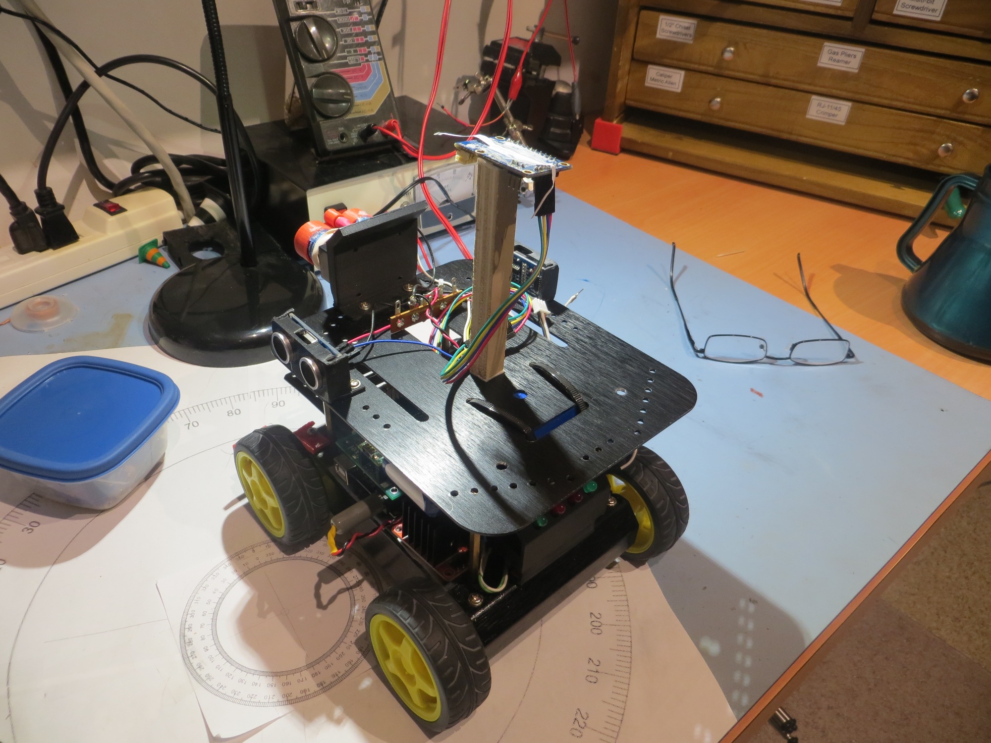
My last post on this subject described my successful effort to mount my Mongoose IMU on Wall-E2, my wall-following robot.  I showed that the IMU, mounted on an 11cm wood stalk on Wall-E2’s top deck, when calibrated using my Magnetometer Calibration tool, provided reasonably accurate and consistent magnetic heading measurements.

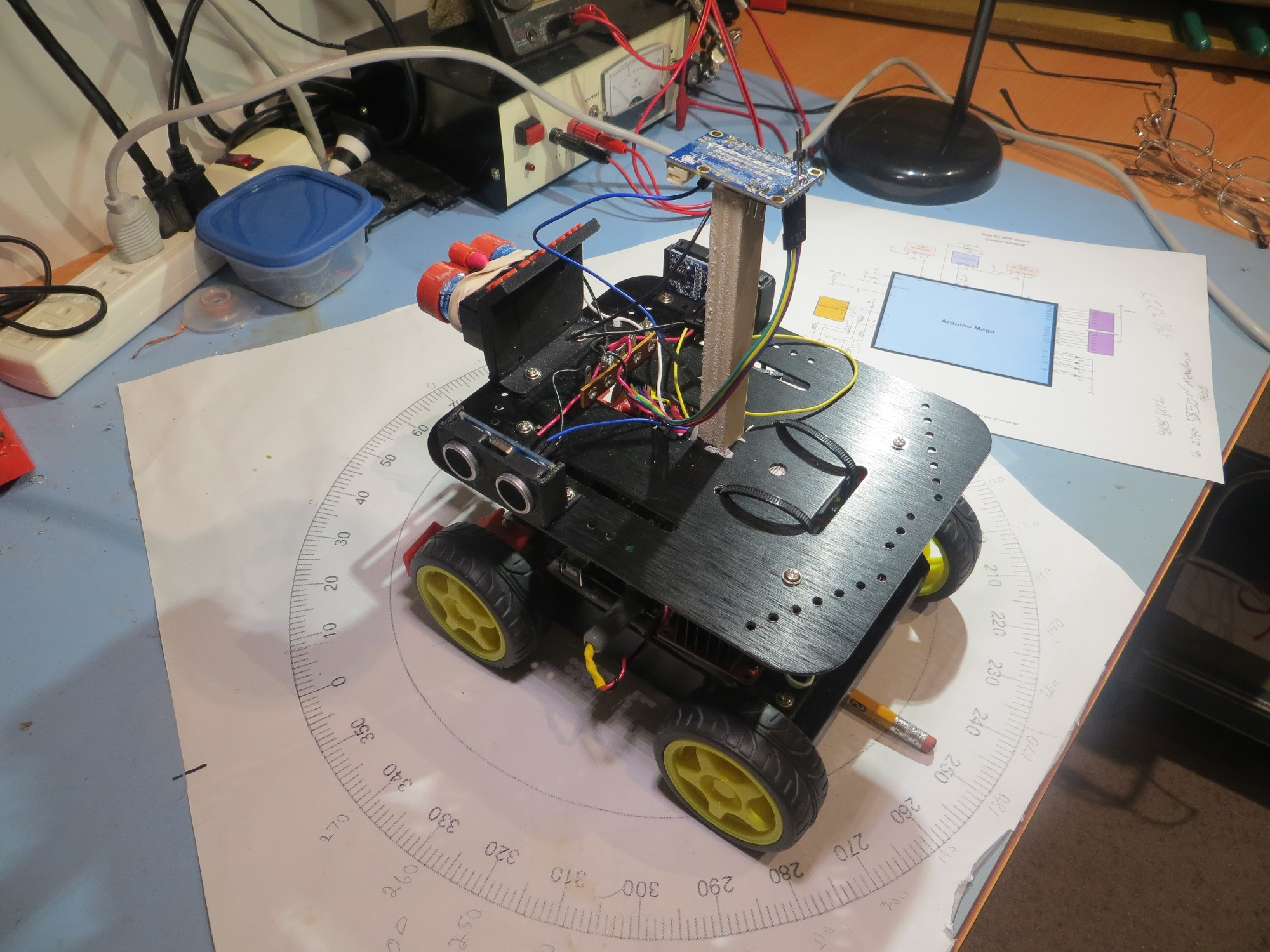
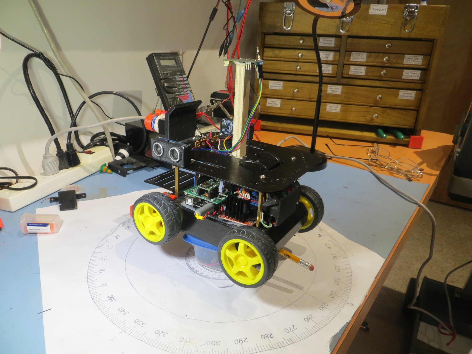
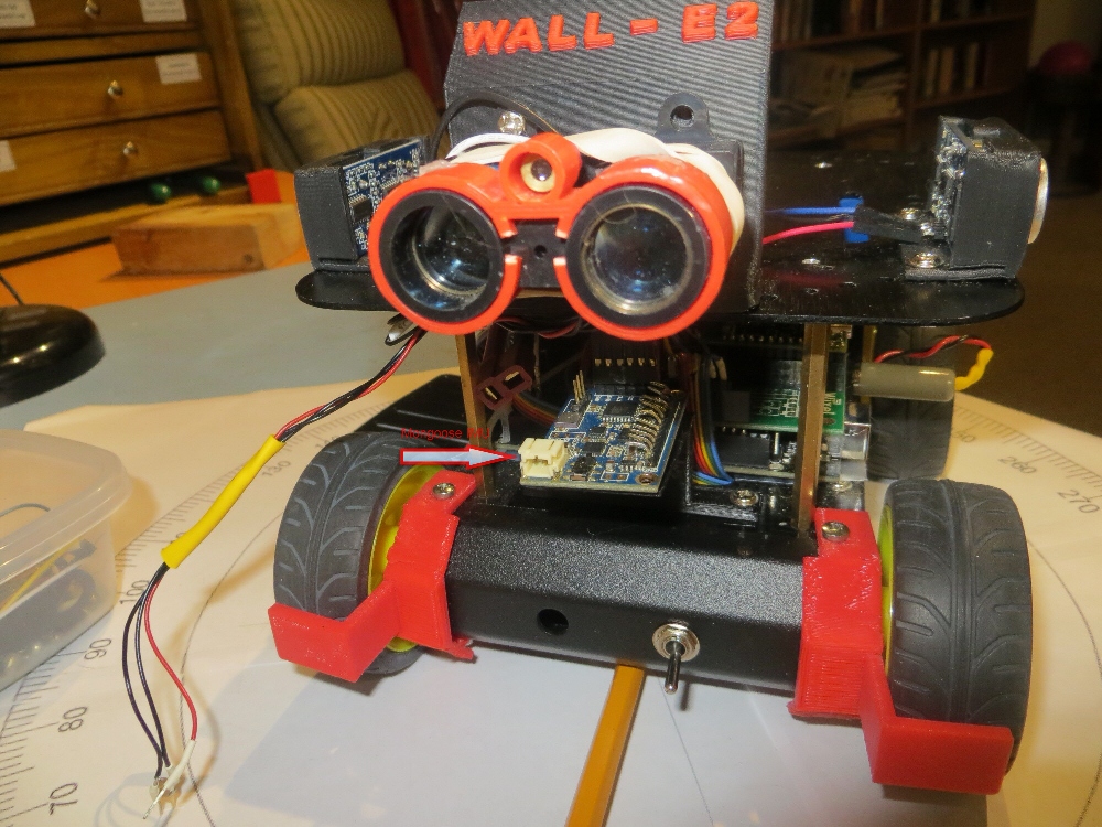
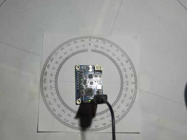
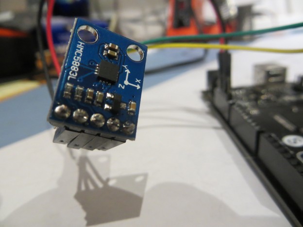
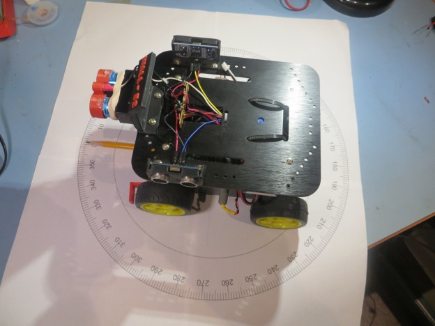
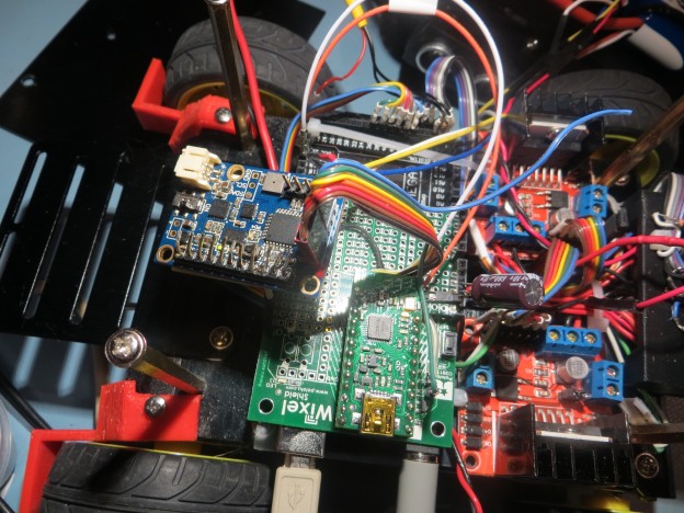
This post attempts to extend these results by replacing the long wooden stalk with a more compact plastic mounting bracket (actually my original IMU mounting bracket) as shown below

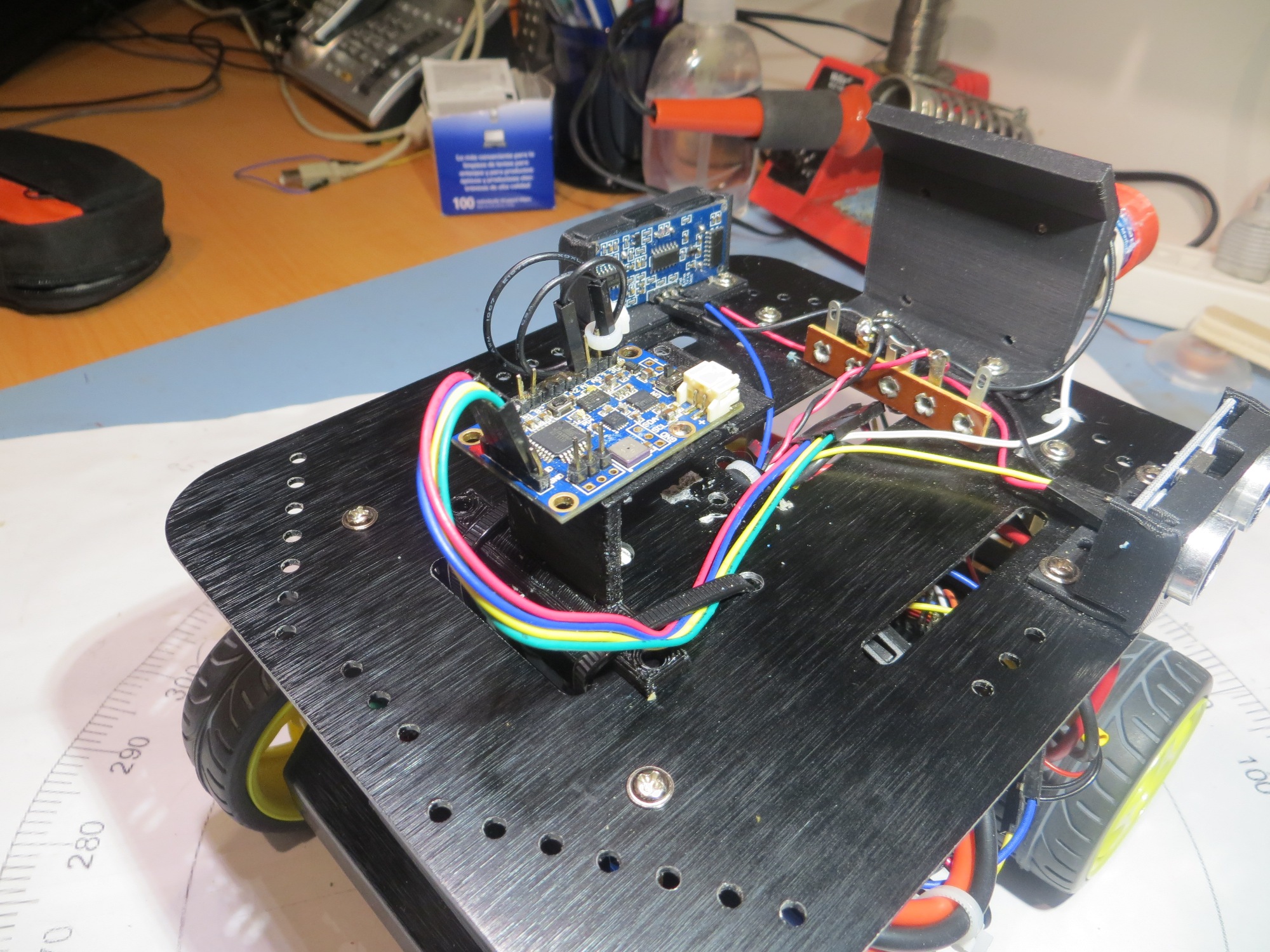
Mongoose IMU mounted on 2nd deck using original mounting bracket

In an effort to determine what, if any, effect the stalk mounting had on IMU calibration, I decided to acquire and plot  calibrated (as opposed to raw) magnetometer data using my mag cal tool, and compare it to the results of the calibration performed on the stalk-mounted configuration.  Since I don’t currently save the ‘calibrated’ point-cloud (there’s no need, as all it does is show how well (or poorly) the raw mag data point cloud is transformed using the generated calibration matrix/center offset values), I first had to import the saved raw data from the stalk-mounted configuration and then regenerate the calibration values (and the resultant ‘calibrated’ point cloud).  Once this was done, then I can capture the new calibrated (i.e. calibrated using the previous stalk-mounted calibration values) but now in the lower mounting position.  If the stalk mounting had no additional isolation effect, the two point clouds should look identical.  If the stalk mounting  did have some effect, then the two clouds should look different.

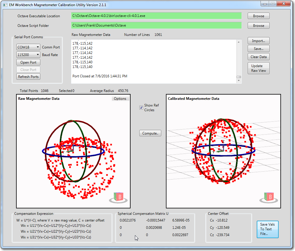
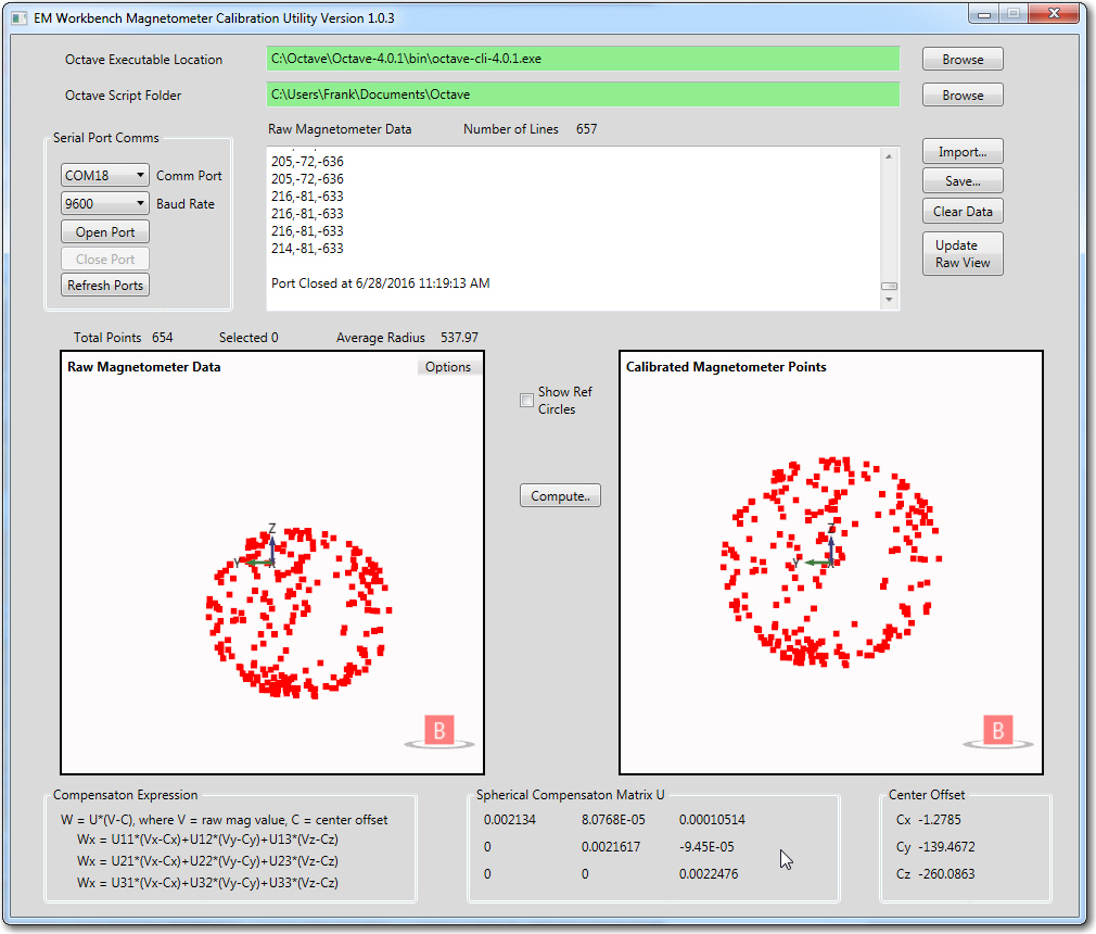
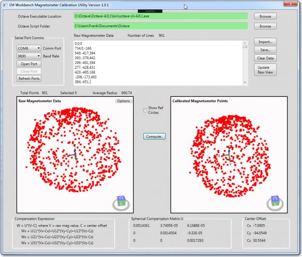
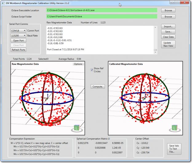
I started by launching the mag cal tool and importing  the raw mag data captured 07/06/16. Then I computed the calibration factors and the resulting ‘calibrated’ point cloud, as shown in the following screenshot.

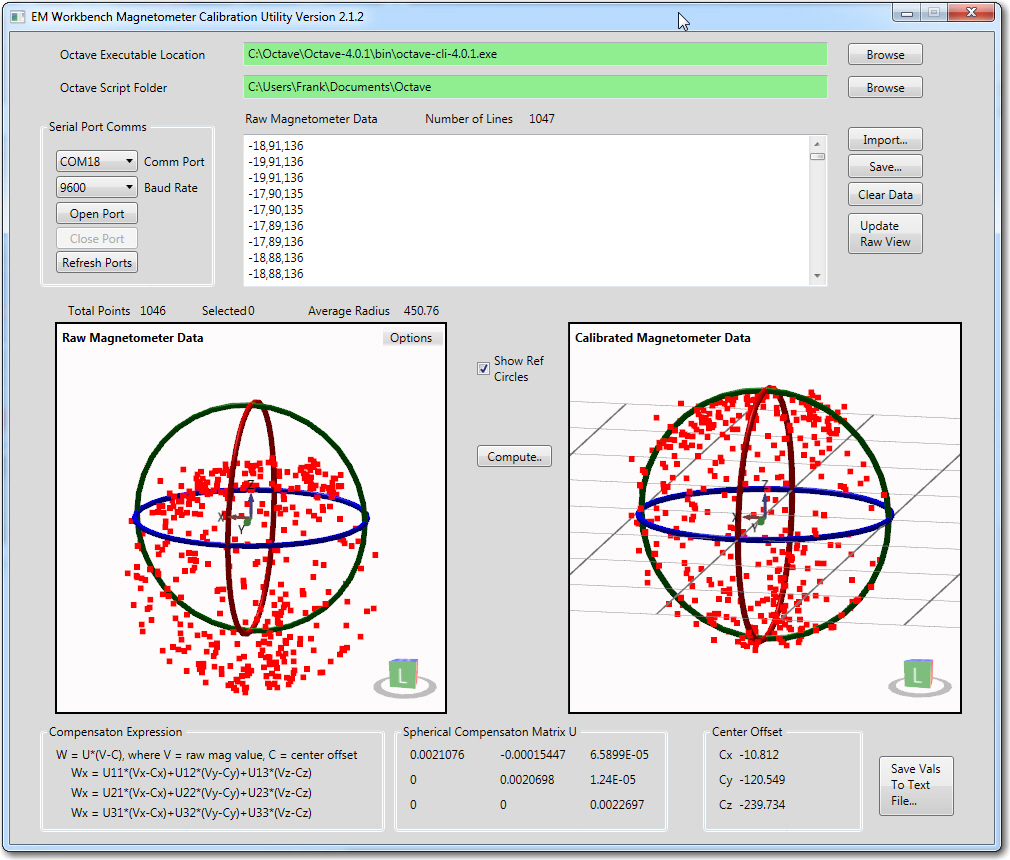
Raw mag data from the stalk-mounted config, and the resulting calibrated point cloud

As can be seen from the image, the data calibrated quite well, starting with a visibly offset point cloud with an average radius of about 450, and ending with a well-centered and symmetric point cloud with a radius close to 1.

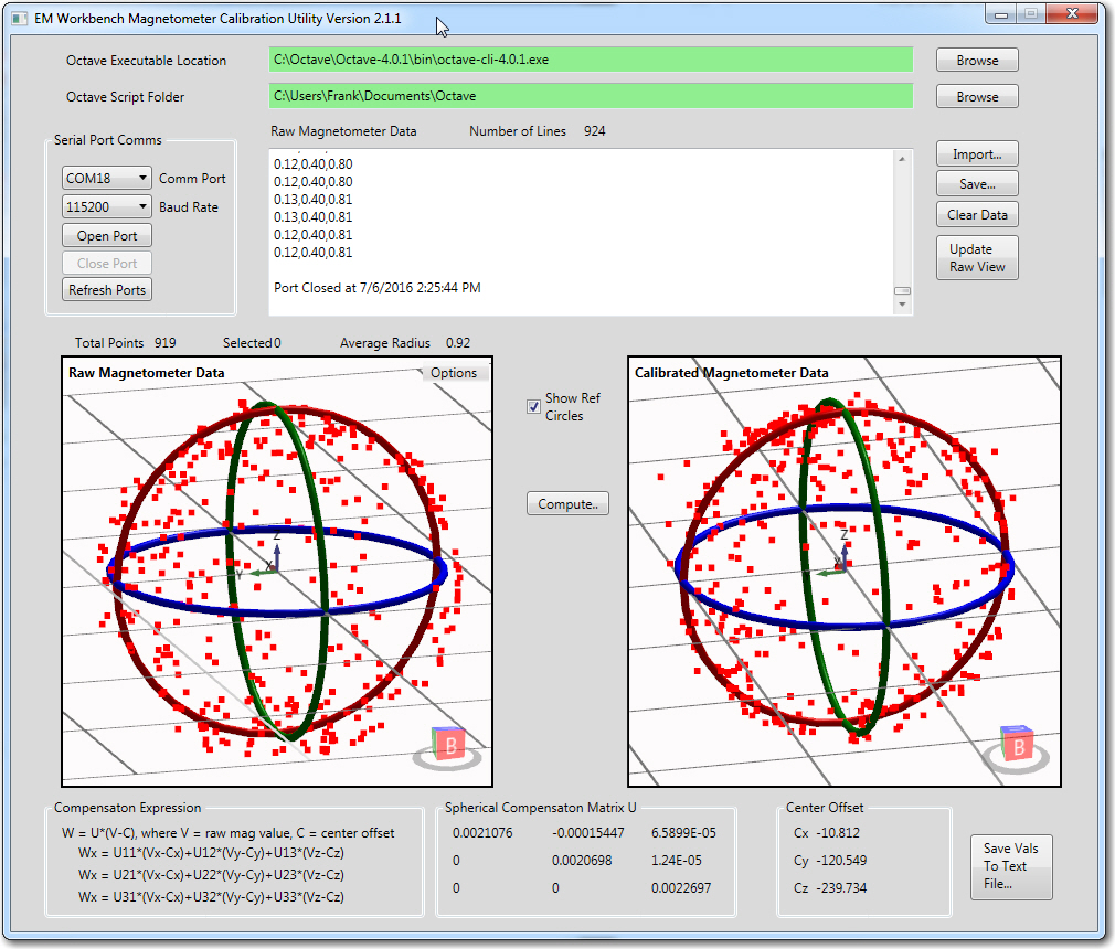
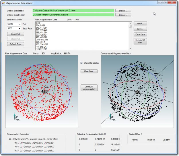
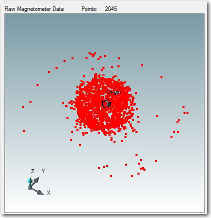
Next, I captured a set of data from the bracket-mounted IMU, using the calibration values from the 6 July stalk-mounted config (this required a bit of reprogramming to pare back the reporting from Wall-E2 to just the magnetometer 3-axis data).  The data was captured by manually rotating Wall-E2 about all 3 axes in a way that produced a well-populated ‘point cloud’ in the mag cal tool app.  During this run, Wall-E2 had power applied, and all motor drives enabled.

Bracket-mounted IMU calibrated magnetometer data vs 06 July stalk-mounted computed calibration data, with Wall-E2 power on and motors running.

From the above screenshot it is quite clear that the stalk and bracket mounting configurations are essentially identical in terms of their calibrated performance.  This means I could, if I so chose, simply use the stalk-mounted calibration values and party on.  Moreover, if I do chose to re-calibrate, I wouldn’t expect to see much change in the calibration values.

Here’s a short movie showing the calibration process:

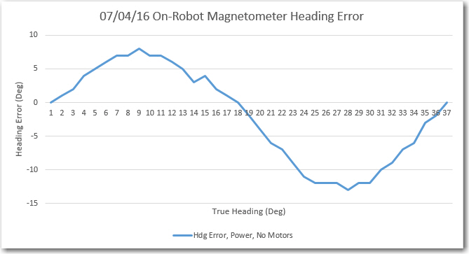
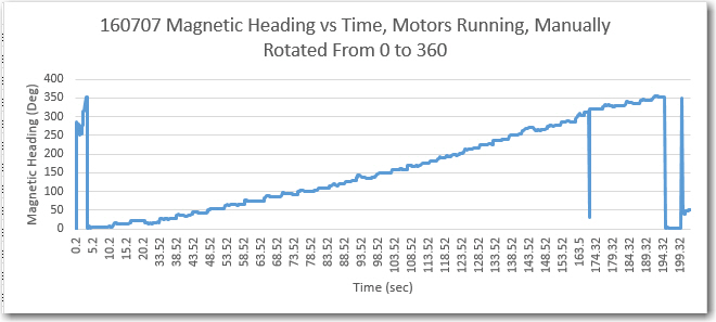
After noting  that the ‘stalk’ calibration values appeared to be reasonably valid for the bracket-mounted configuration, I re-ran the heading error tests on my bench-top heading range, with the following results:

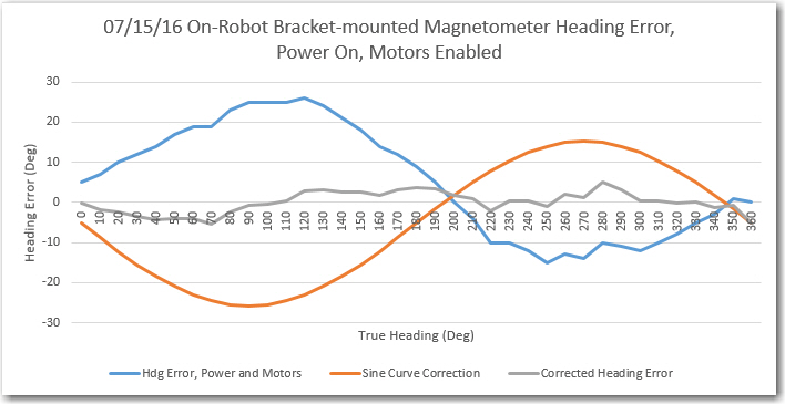
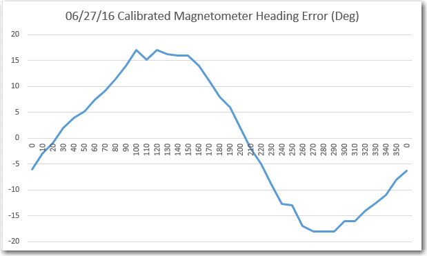
Bracket-mounted IMU Heading Error, Power On, Motors Running

For comparison, here is the ‘stalk’ heading error chart

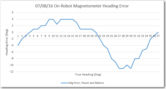
Stalk-mounted Mongoose IMU, with power and motor drive enabled.

And the original problem measurement from back in March with the IMU mounted on the first deck at the front of the robot:

Heading performance for front-mounted IMU, power off.

From the above, it is kind of hard for me to believe that this much error could possibly be corrected just via the calibration matrix and center offset adjustments, so I suspect the current performance depends as much on moving the IMU from directly over the front motors to the 2nd deck (a minimum of 10cm from the rear motors, and about 15 from the front ones) as it does on the calibration values.  I could verify this by re-mounting the IMU on the front and seeing if I could calibrate out the errors, but I’d rather let sleeping dogs lie at this point ;-).

Frank

Posted July 06, 2016

In my last post  on this subject, I had used my newly-completed Magnetometer Calibration Tool to generate calibration factors for my HMC5883L-based ‘Mongoose IMU board, and compare the ‘raw’ vs ‘calibrated’ performance in a ‘free-space’ (actually my wood lab workbench) environment.  The result of the comparison showed  that the  ‘calibrated’ performance was pretty much unchanged from the ‘raw’ setup, indicating that the test setup (on my wooden workbench) wasn’t significantly affected by ‘hard’ or ‘soft’ interference.

The next step is to mount the Mongoose IMU on Wall-E2, my 4WD wall-tracking robot to see if the magnetometer can be compensated for DC motor magnet fields, power cables, and the like.  I decided to start this process by mounting the IMU on a wooden ‘stalk’ on the second deck, to see if this placement would minimize the above interfering effects.

Mongoose IMU mounted on wooden stalk on 2nd deck

Raw and calibrated data. Reference circles on left have radii equal to average raw value radius. Circles on right all have a radius == 1

The calibration values can now be saved to a text file convenient for transcription into the user’s calibration routine.  After doing the save, the text file looks like the following;

After copy/pasting the above values into my calibration routine and re-running the data collection exercise but recording the calibrated magnetometer readings instead, I got the following ‘raw’ (calibrated magnetometer data, but displayed in the ‘raw’ view) results.

Comparison of new calibrated data from the magnetometer with the results of the Octave calibration algorithm as applied to the old set of raw magnetometer data.

The displayed data in the ‘raw’ view is new magnetometer data after being calibrated with the results of the first run. The circle radius on the left is 0.92. The data on the left is the old magnetometer data, calibtrated using the results of the calibration value computation from the first set of raw magnetometer data.  As is easily seen from the two views, the calibration values generated by the Octave program produce very good ‘on-the-fly’ calibration results.

After calibration, I re-ran the heading performance tests (main power ON, but no drive to the motors), with the following results

Stalk-mounted magnetometer heading error, main power, no motor drive

The next step is to repeat this experiment with the motor drives enabled.  Here’s the results of a quick run.  With the motors enabled, I held Wall-E2 so that it’s wheels didn’t quite touch the surface, and slowly rotated the robot 360 clockwise, starting at the same point (nominally 0 deg as reported by the Mongoose IMU) as in the above plot.

Manually rotated over 360 degrees with motors running. Mongoose stalk mounted on 2nd deck

As shown in the plot above, the headings reported by the Mongoose IMU increased monotonically as the robot was rotated clockwise from nominal zero. Although just a preliminary result, it  is actually quite encouraging, as it indicates that running the motors doesn’t significantly affect the heading value reported by the Mongoose IMU.

Today I had the chance to perform a ‘motors running’ heading error experiment with the stalk-mounted Mongoose IMU.  The robot body was placed on a small plastic box such that the wheels were free to turn without touching the workbench.  Then it was manually rotated in 10 deg increments as before.  The experimental setup and the results are shown below.

Test setup for the “Power and Motors” IMU heading error experiment.

Stalk-mounted Mongoose IMU, with power and motor drive enabled.

Comparing the heading error plots, it is pretty clear that enabling the motors does not significantly affect the stalk-mounted IMU.  If I wanted to leave the IMU mounted on the stalk, it appears that I could expect to get reasonable, if not spectacularly accurate, magnetic heading readings ‘in real life’.

However, I really  don’t want to leave the IMU mounted on a stalk, so the next step in the process will be to replace the stalk mounting arrangement with a more ‘streamlined’ mounting setup.  For this I plan to use the mounting bracket I printed up for the original front-mounted setup (see image below), but attached to the 2nd deck vs the 1st.

Original mounting location for the Moongoose IMU (arrow points to the IMU)

Posted 06/18/16

My last few posts have described my efforts to create an easy-to-use magnetometer calibration utility to allow for as-installed  magnetometer calibration.  In situ calibration is necessary for magnetometers because they can be significantly affected by nearby ‘hard’ and ‘soft’ iron interferers.  In my research on this topic, I discovered there were two main magnetometer calibration methods; in one, 3-axis magnetometer data is acquired with the entire assembly containing the magnetometer placed in a small but complete number of well-known positions.  The data is then manipulated to generate calibration values that are then used to convert magnetometer data at an arbitrary position.  The other method involves  acquiring a large amount (hundreds or thousands of points) of data while the assembly is rotated arbitrarily around all three axes.  The compensation method assumes the acquired data is sufficiently varied to cover the entire 3D sphere, and then finds the best fit of the data to a perfect sphere centered at the origin.  This produces an upper triangular 3×3 matrix of multiplicative values and an offset vector that can be used to convert any magnetometer position raw value to a compensated one.  I decided to create a tool using the second method, mainly because I had available a MATLAB script that would do most of the work for me, and Octave, the free open-source application that can execute most MATLAB scripts.  Moreover, Octave for windows can be called from C#/.NET programs, making it a natural fit for my needs.  In any case, I was able to implement the utility (twice!!) over the course of a couple of months, getting it to the point where I am now ready to try calibrating my CK Devices ‘Mongoose’ IMU, as installed on my ‘Wall-E2’ four-wheel drive robot.

However, before mounting the IMU on the robot and going for ‘the big Kahuna’ result, I decided to essentially re-create my original experiment with the IMU rotated in the X-Y plane on my bench-top, as described in the post ‘Giving Wall-E2 A Sense of Direction – Part III‘.  My 4-inch compass rose had long since bitten the dust, but I had saved the print file (did I tell you that I  never throw anything away)

Mongoose IMU on 4-Inch Compass Rose

So, I basically re-created the original heading error test from back in March, and got similar (but not identical) results, as shown below:

Heading Error, Compensation, and Comp+Error

06/19/16 Mongoose ‘Desktop’ Heading Error

Then I used my newly minted magnetometer calibration utility to generate a calibration matrix and center offset, so I can apply them  to the above data.  However, before I can do that I have to go back into CK Devices original code to find out where the calibration should be applied – more digging :-(.

In the original Mongoose IMU code, the function ‘ReadCompass()’ in HMC5883L.ino gets the raw values from the magnetometer  and  generates compensated values using whatever values the user places in two ‘struct’ objects (all zeros by default).  However, I was clever enough to only send the ‘raw’ uncalibrated magnetometer data to the serial port, so that is what I’ve been using as ‘raw’ data for my mag calibration tool – so far, so good.  However, what I need for my robot is compensated values, so (hopefully) I can (accurately?) determine Wall-E2’s heading.

So, it appears I have two options here; I can continue to emit ‘raw’ data from the Mongoose and perform any needed compensation externally, or I can do the compensation internally to the Mongoose and emit only corrected mag data.  The problem with the latter option (internal to the Mongoose) is that I would have to defeat it each time the robot configuration changed, with it’s inevitable change to the magnetometer’s surroundings.  If I write an external routine to do the compensation based on the results from the calibration tool, then it is only that one routine that will require an update.  OTOH, If the compensation is internal to the Mongoose, then modularity is maximized – a very good feature.  The deciding factor is that if the routine is internal to the Moongoose, then I can remove it from the robot and I still have a complete setup for magnetometer work.  So, I decided to write it into the Mongoose code,  but have the ability to switch it in/out with a compile time switch (something like NO_MAGCOMP?)

The compensation expression being implemented is:

W = U*(V-C), where U = spherical compensation matrix, V = raw mag values, C = center offset value

Since U is always upper triangular (don’t ask – I don’t know why), the above matrix expression simplifies to:

Wx = U11*(Vx-Cx) + U12*(Vy-Cy) + U13*(Vz-Cz)
Wy = U22*(Vy-Cy) + U23*(Vz-Cz)
Wz = U33*(Vz-Cz)

I implemented the above expression in the Mongoose firmware by adding a new function ‘CalibrateMagData()’ as follows:

Using the already existing s_sensor_data struct which is defined as follows:

Then I created another ‘print’ routine, ‘PrintMagCalData()’ to print out the calibrated (vs raw) magnetometer data. Also, after an overnight dream-state ‘aha’ moment, I realized I don’t have to incorporate a compile-time #ifdef statement to switch between ‘raw’ and ‘calibrated’ data readout from the Mongoose – I simply attach a jumper from either GND or +3.3V to one of the I/O pins, and implement code that calls either ‘PrintMagCalData()’ or ‘PrintMagRawData()’ depending on the HIGH/LOW state of the monitor pin. Now  that’s elegant! 😉

After making these changes, I fired up just the Mongoose using VS2015 in debug mode, which includes a port monitor function.  As soon as the Moongoose came up, it started spitting out 3D magnetometer data – YAY!!

It’s been a few days since I got this going – my wife and I went off to a weekend bridge tournament in Kentucky and we got back late last night – so I didn’t get  a chance to compare the ‘after-calibration’ heading performance with the ‘before’ version until today.

After Calibration Magnetic Heading Error

Comparing the above chart to the one from 6/19, it is clear that they are virtually identical.  I guess what this means is that, at least for the ‘free space’ case with no nearby interferers, calibration doesn’t do much.  Also, this implies that the heading errors observed above have nothing to do with external influences – they are ‘baked in’ to the magnetometer itself. The good news is, a sine function correction table should take most of this error out, assuming more accurate heading measurements are required (I don’t ).

In summary, at this point I have a working magnetometer calibration tool, and I have used it successfully to generate calibration matrix/center offset values for my Mongoose IMU’s HMC5883 magnetometer component.  After calibration, the ‘free space’ heading performance is essentially unchanged, as there were no significant ‘hard’ or ‘soft’ iron interferers to calibrate out.

Next up – remount the Mongoose on my 4WD robot, where there are  plenty of hard/soft iron interference sources, and see whether or not calibration is useful.

posted 06/14/16

In my last post on the subject of Magnetometer Calibration, I described an entirely complete and wonderful calibration utility I wrote in C#/.NET using Windows Forms, an old version of devDept’s EyeShot 3D viewport library, and calls into the Octave libraries to execute a MATLAB calibration script.  Unfortunately, at the end of the project I discovered to my horror that my redistribution rights for the EyeShot libraries had expired some time ago, and re-upping them was prohibitively expensive – so I could use my masterpiece, but no one else could! :-(.

So, it was ‘back to the drawing board‘ for me.  I needed a (ideally free) 3D visualization capability with reasonably easy-to-implement  view manipulation (pan, zoom, rotate, coordinate axis, etc) tools that was compatible with C#/.NET.    After a fair bit of research, I found that Microsoft’s WPF (Windows Presentation Framework) platform advertised ‘full’ 3D visualization capability, so that was encouraging. Unfortunately, I had never used WPF at all, doing all my C#/.NET programming in the Windows.Forms namespace.  There were some posts that suggested the ability to place  a WPF 3D viewport window into a Forms-based app via a ‘WindowsFormsHostingWpfControl’ but after trying this a bit I decided it was going to be too hard to build up the required 3D viewport and associated view manipulation tools ‘from scratch’.  Eventually I ran across the 3D Helix Toolkit at  http://www.helix-toolkit.org/, and this looked very promising, but with the downside of having to re-create the entire application in WPF-land.  Actually, this appealed to me in a masochistic sort of way, as I would have the opportunity to learn two completely new packages/skills – WPF programming in general (which I had been ignoring for years in the hopes it would go away) and the feature-rich (but somewhat rough around the edges) Helix Toolkit.

So, off I went, reading as much as I could get my hands on about WPF and .NET visual programming.  It was initially very difficult to wrap my head around the way that WPF combines XAML with C# ‘code-behind’ to achieve the desired results.  At first I started out trying desperately to stick to my WinForms technique of drag/dropping tools onto a work surface, and then modifying properties as desired.  This worked up to a point, but I rapidly got lost due to the marked difference between WinForm’s ‘everything is a child of the main window’ and WPF’s hierarchical layout as described in XAML philosophy.  So, my first effort to build a WPF app isn’t very pretty, and  definitely violates any number of rules for WPF elegance!  However, the use of WPF and the Helix Toolkit made it reasonably easy to implement the ‘raw’ and ‘calibrated 3D views, and I had no real trouble porting the comm port and Octave implementation logic from my previous app to this one.  And of course, the entire object of the exercise was to create an app that could be shared, and the WPF version (hopefully) does that.

My plan for the future – at least with respect to the Magnetometer Calibration Utility, is to share the app within the robotics/drone community, and to continue to support  it as necessary to fix bugs and/or implement requested enhancements.  I also plan to set up a public GitHub repository as soon as I can figure out how to do it ;-).

Posted 06/13/16

In my last post on this subject back in April, I had managed to figure out that my feeble attempts to compensate my on-robot magnetometer for hard/soft iron errors wasn’t going to work, and I was going to have to actually do a ‘whole sphere’ calibration to get any meaningful azimuth values from my magnetometer as installed on my robot.

As noted back in April, I had discovered two different tools for full-sphere magnetometer calibration (Yuri Matselenak’s program from the DIY Drones site, and Alain Barraud’s MATLAB script from 2008), but neither of them really filled the bill for an easy-to-use GUI for dummies like me.  At the end of April’s post, I had actually built up a partial GUI based on devDept’s EyeShot 3D viewport technology that I had lying around from a previous lifetime as a scientific software developer.  All I had to do to complete the project was to figure out how to integrate Alain’s MATLAB code into the EyeShot-based GUI and I’d be all set – or so I thought! ;-).

Between that last post in April and now, I have been busy with various insanities – competitive bridge, trying to develop a 3-point basketball shot, and generally screwing off, but I did manage to spend some time researching the issue of MATLAB-to-C# code porting.  At first I thought I would be able to simply port the MATLAB code to C# line-by-line.  I had done this in the past with some computational electromagnetics codes, so how hard could it be, anyway?  Well, I found out that it was pretty fricking hard, as in effectively impossible – at least for me; I just couldn’t figure out how to relate  the advanced matrix manipulations in Alain’s code to the available math tools in C#.  I even downloaded the Math.NET Numerics toolkit from  http://numerics.mathdotnet.com/ and tried it for a while, but I just could not make the connection between MATLAB matrix manipulation concepts and the corresponding ones in the Numerics toolkit – argghhh!!!.

After failing miserably, I decided to try and skin the MATLAB cat a different way.  I researched the Gnu Octave community, and discovered that not only was there a nice Octave GUI available for windows, but that some developers had been successful at making calls into the Octave dll’s from C# .NET code – exactly what I needed!

So, it was full steam ahead (well, that’s not saying much for me, but…) with the idea of a C#.NET GUI that used my EyeShot 3D viewport for visualization, and Octave calls for the compensation math, and  within a few weeks I had the whole thing up and running – a real thing of beauty that I wouldn’t mind sharing with the world, as shown in the following video clip.

Unfortunately, after doing all this work I discovered that my EyeShot redistribution license for the 3D viewport library had long since expired, and although I can run the program happily on my laptop, I can’t distribute the libraries anywhere :-(((((.

Ah, well, back to the drawing board!

Frank

(author’s note: Although I did this work back in the April/May timeframe, I didn’t post about it until now.  I decided to go ahead and post it  now as a ‘prequel’ to the next post about my ‘final solution’ to the magnetometer calibration utility challenge)

Posted 20 April, 2016

I have been trying to add a magnetometer to my Wall-E2 robot for a while now, and have been plagued by installation-induced errors.  A magnetometer works fine on the bench in isolation, but not when installed on the robot.  So far, I have determined that the DC drive motors are a big contributor to these errors, and the only way to address this is with magnetometer calibration.  At first I tried just a simple lookup-table based approach, since I only needed to correct for azimuth errors (my wheeled robot very rarely departs from a horizontal orientation).  Again, this worked great ‘on the bench’, but failed miserably in the installed configuration.

So, after being forcibly convinced that ‘the easy way’ wasn’t going to work, I began researching magnetometer calibration techniques and tools.  At the DIY Drones website, I found a very informative article by Yury Matselenak  with a great explanation, and a set of two tools (a visualizer and a calibration tool).  I thought I was ‘in like Flynn’ and downloaded the tools.  Unfortunately the visualizer tool didn’t recognize comm two-digit port port numbers, so once again I was stuck (Yuri later gave me a link to the visualizer source code, but I haven’t yet had the time to fix it for the higher numbered ports).  In the meantime, I found another calibration tool, written in MATLAB by Alain Barraud, so I decided to try my hand at a magnetometer calibration manager.  I have a fair bit of experience with MATLAB from a prior lifetime as a researcher, and I have previously ported MATLAB code to C++, so how hard could it be?  From a previous project I had access to an older version the neat EyeShot 3D visualization libraries, so it was easy to add a 3D viewport to a standard C# Windows form.  My plan was to have a ‘raw’ and a ‘calibrated’ view, so it would be easy to see the effects of the calibration process, and to use the free MathNet.Numerics matrix manipulation tools to port the MATLAB code.  Unfortunately, the  MATLAB matrix manipulation routines used in the calibration code didn’t correspond closely enough to  MathNet’s library functions, so I got stuck during the port and wasn’t able to finish the ‘calibrated’ side of the application – bummer!

However, I did get far enough along to notice another problem; the raw data from my magnetometer exhibited a lot of ‘spread’ in one of the principal planes, where a small percentage of the data points formed a rough circle at about twice the radius as all the other points.  When I ran this dataset through Alain’s original MATLAB code (using Octave on my Linux box) the ‘calibrated’ dataset actually looked worse than the original.  This prompted me to add some point editing capability to my visualizer, so I could visually remove ‘outrider’ data prior to attempting calibration.

Raw vs Calibrated data before pruning outliers

Raw vs Calibrated data after pruning outliers

Here are some shots of the process of pruning the dataset using my calibration app

Raw magnetometer data before any pruning

All data beyond a settable radius selected

All selected outliers removed

Pruned data written to text file for later processing through MATLAB calibration app

So, even though I couldn’t (and still can’t) figure out how to port Alain’s MATLAB code into my calibration tool, I  was able to use the tool to visually prune outliers from my data prior to running it through the calibration routine, and so all my work wasn’t a complete waste – whoopee! (not).

Frank