Posted June 16, 2015
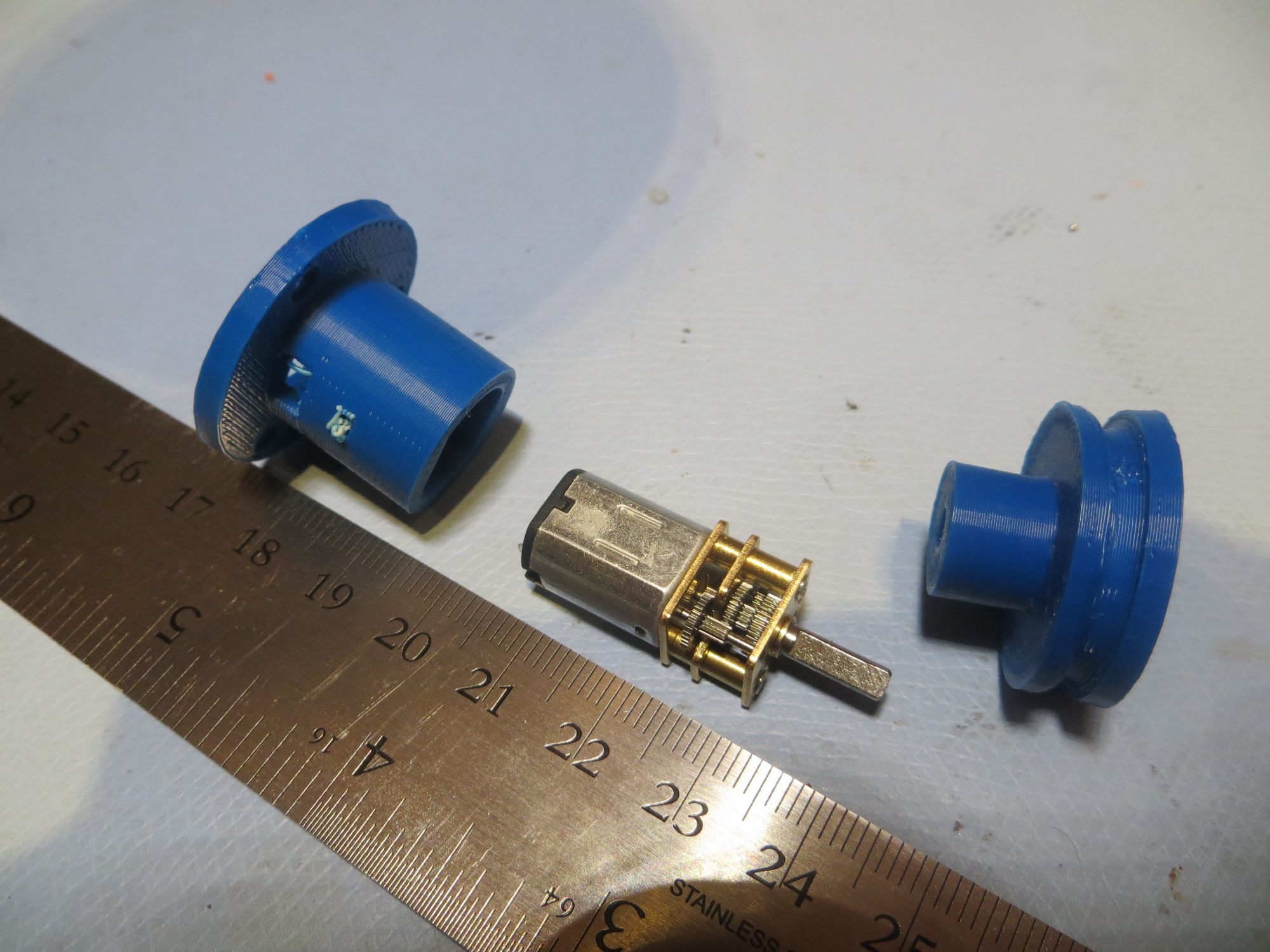
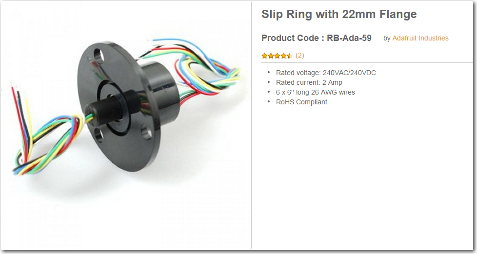
In my last post (http://gfpbridge.com/2015/05/lidar-lite-rotates/ – over a month ago – wow!) I described the successful attempt to mate the Pulsed Lite LIDAR with a 6-channel slip ring to form a spinning LIDAR system for my Wall-E wall-following robot. As an expedient, I used one of Wall-E’s wheel motors as the drive for the spinning LIDAR system, but of course I can’t do that for the final system. So, I dived back into Google and, after some research, came up with a really small but quite powerful geared DC motor rated for 100 RPM at 6 VDC (In the image below, keep in mind that the shaft is just 3mm in diameter!)
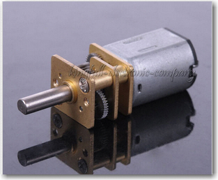
Very small 100RPM geared DC motor. See http://www.ebay.com/itm/1Pcs-6V-100RPM-Micro-Torque-Gear-Box-Motor-New-/291368242712
In my previous work, I had worked out many of the conceptual challenges with the use of an offset motor, O-ring drive belt, and slip ring, so now the ‘only’ challenge was how to replace Wall-E’s temporarily-borrowed wheel motor with this little gem, and then somehow integrate the whole thing onto the robot chassis.
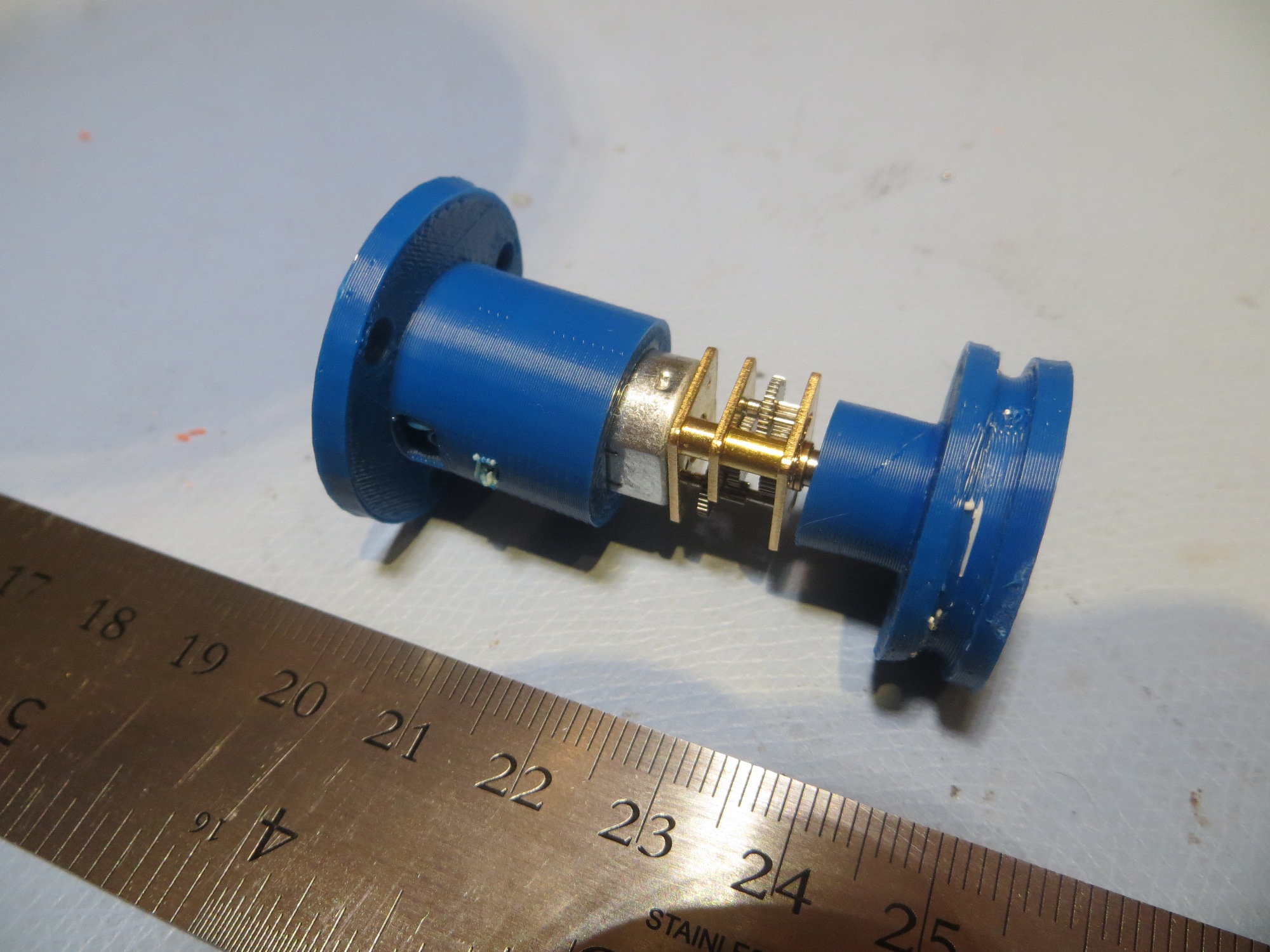
The first thing I did was come up with a TinkerCad design for mounting the micro-motor on the robot chassis, and the pulley assembly from the previous study onto the motor shaft. Wall-E’s wheel motor has a 6mm shaft, but the micro-motor’s shaft is only 3mm, so that was the first challenge. Without thinking it through, I decided to simply replace the center section of the previous pulley design with a center section sporting a 3mm ‘D’ hole. This worked, but turned out to be inelegant and WAY too hard. What I should have done is to print up a 3mm-to-6mm shaft adapter and then simply use all the original gear – but no, I had to do it the hard way! Instead of just adding one new design (the 3mm-to-6mm adapter), I wound up redesigning both the pulley and the tach wheel – numerous times because of course the first attempts at the 3mm ‘D’ hole were either too large or too small – UGGGGGHHHH!!
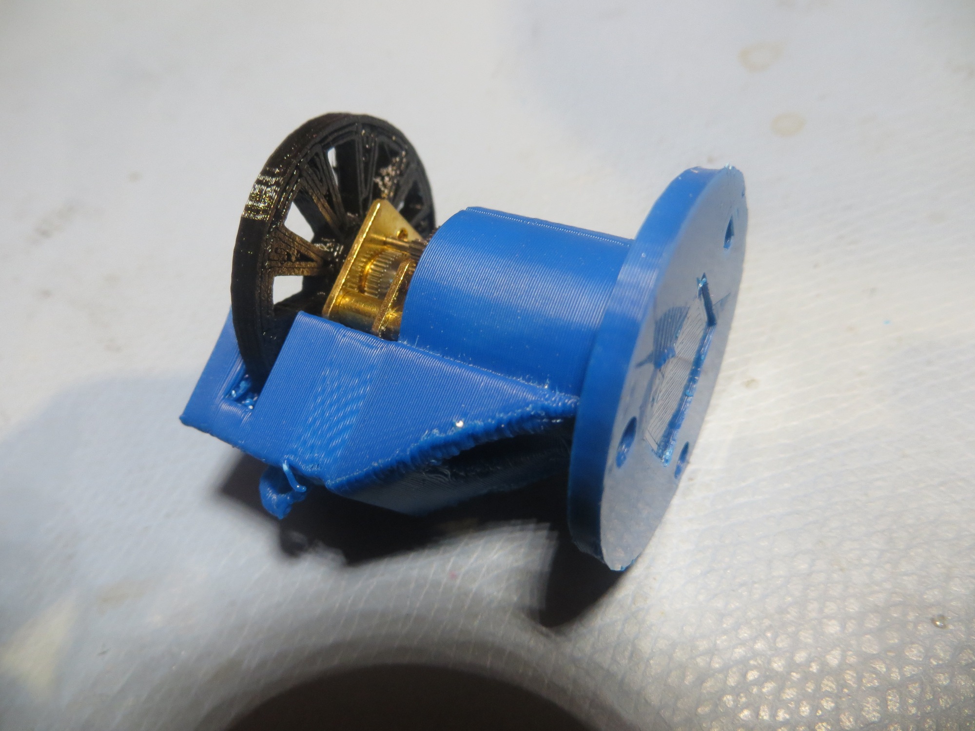
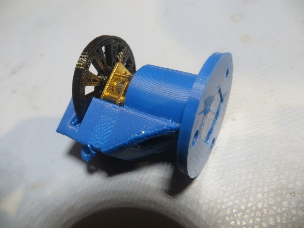
Anyway, the motor mount and re-engineered pulley/tach wheel eventually came to pass, as shown below. I started with a basic design with just a ‘cup’ for the motor and a simple drive belt pulley. Then I decided to get fancy and incorporate a tach wheel and tach sensor assembly into the design. Rather than having a separate part for the sensor assembly, I decided to integrate the tach sensor assembly right into the motor mount/cup. This seemed terribly clever, right up until the point when I realized there was no way to get the tach wheel onto the shaft and into the tach sensor slot – simultaneously :-(. So, I had to redesign the motor ‘cup’ into a motor ‘sleeve’ so the motor could be slid out of the way, the tach wheel inserted into the tach sensor slot, and then the motor shaft inserted into the tach wheel ‘D’ hole – OOPS! ;-).

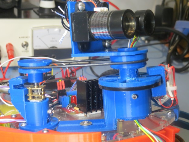
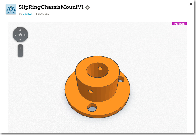
Assembled Miniature DC Motor Mount

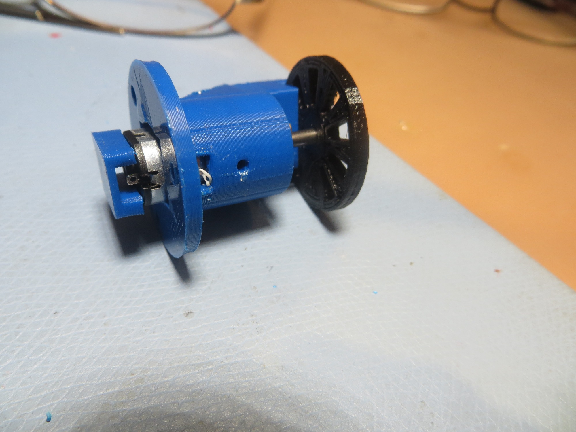
Miniature DC motor with chassis mount and belt drive wheel

Miniature DC motor partially installed in chassis mount
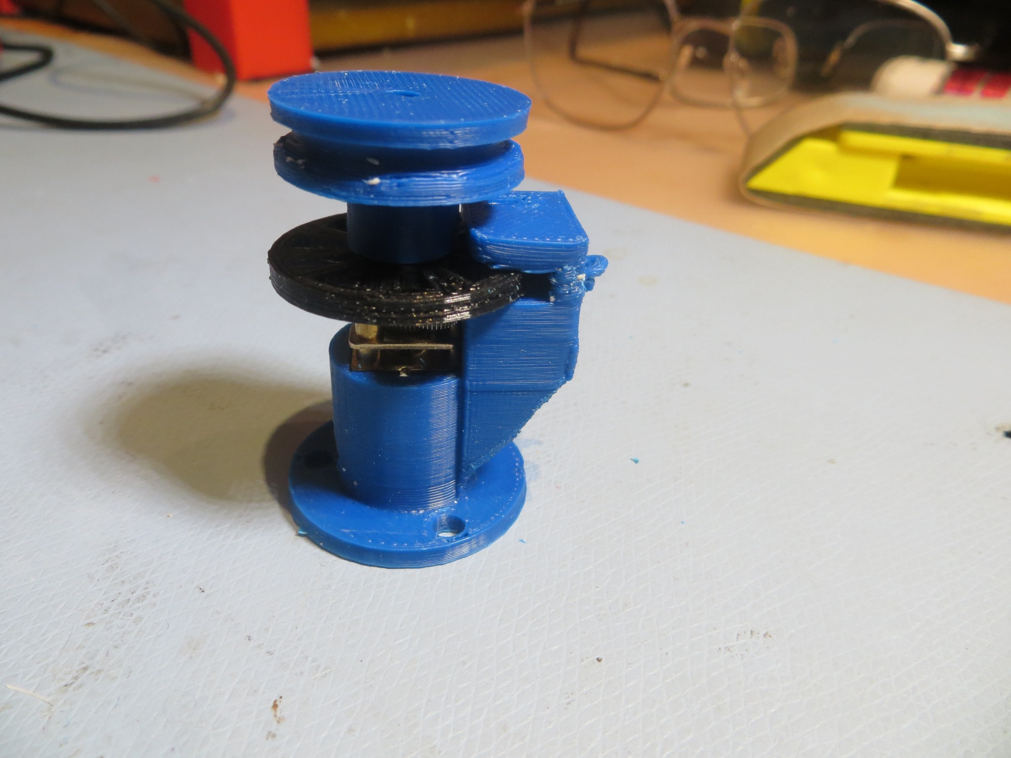
Miniature DC motor mount, with tach sensor attachment, side/bottom view

Miniature DC motor mount, with tach sensor attachment, side view showing motor contact cover
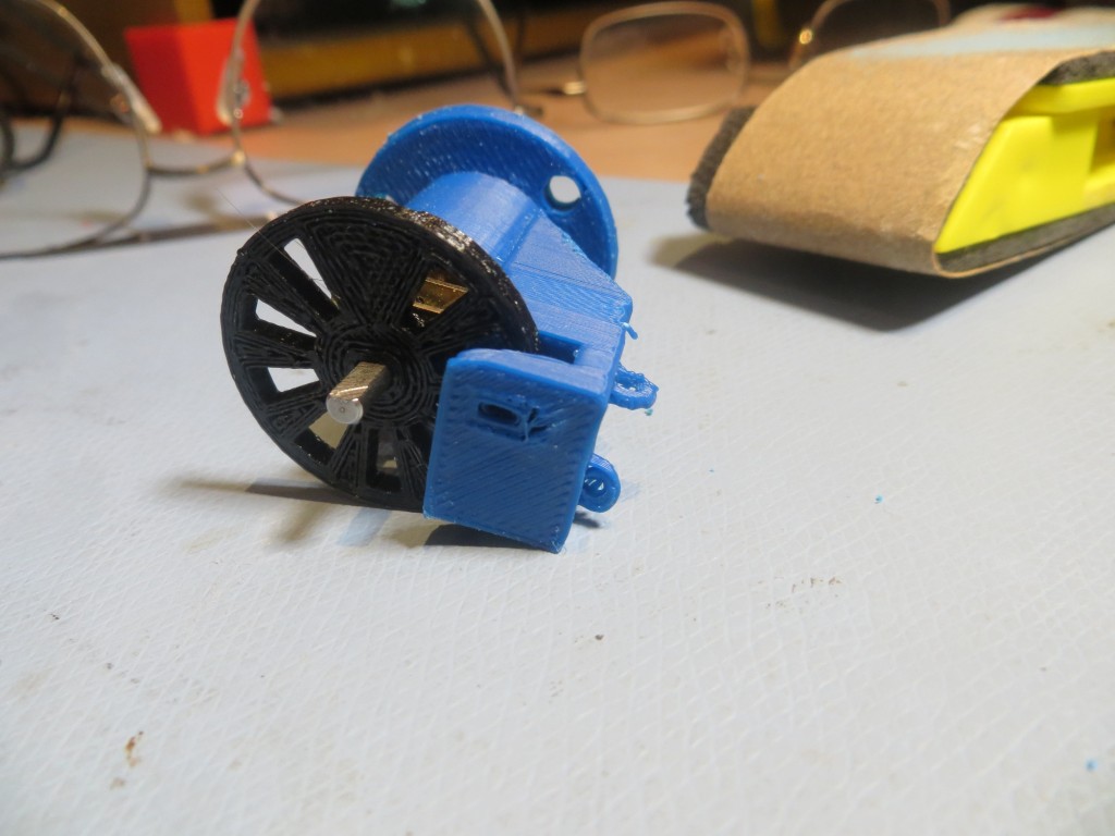
Miniature DC motor mount, with tach sensor attachment, top view
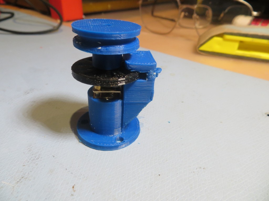
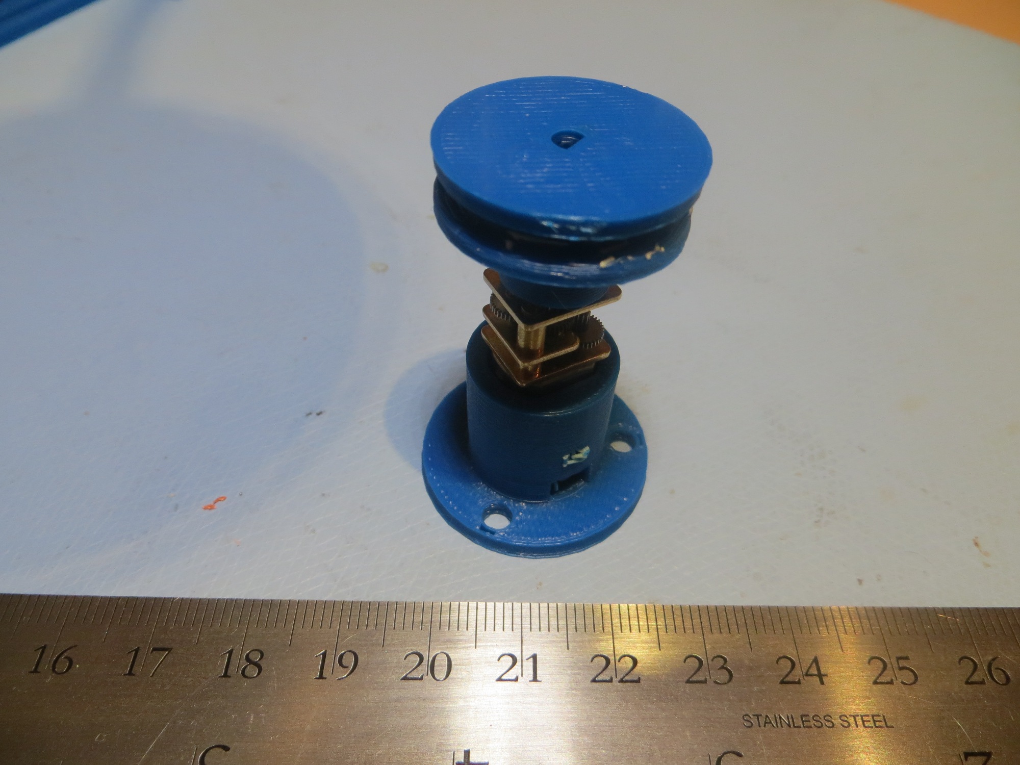
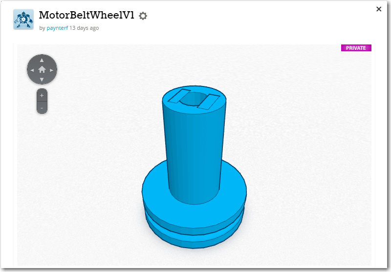
Completed assembly, with drive belt pulley and tach wheel
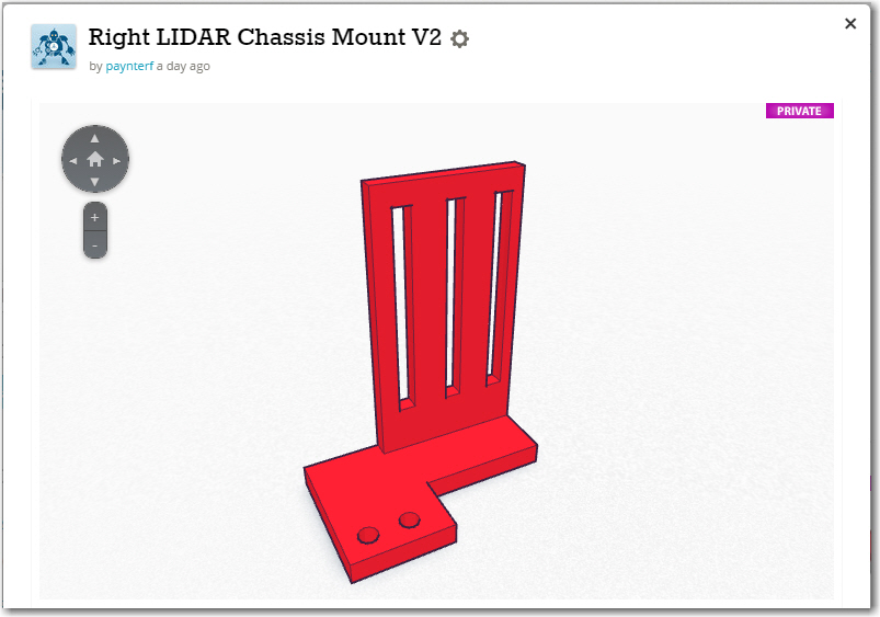
Next up – the LIDAR mount. The idea was to mount the LIDAR on the ‘big’ side of the 6-channel slip ring assembly, and do something on the ‘small’ side to allow the whole thing to slide toward/away from the motor mount to adjust the drive belt tension. As usual, I didn’t have a clue how to accomplish this, but the combination of TinkerCad and 3D printing allowed me to evolve a workable design over a series of trials. The photo below shows the LIDAR mounted on the ‘big’ side of the slip ring, along with several steps in the evolution of the lower slide chassis mount
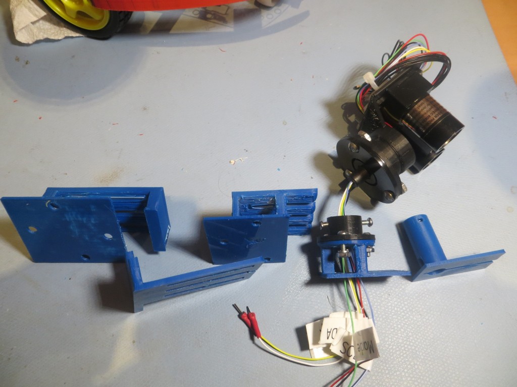
Evolution of the slide mount for the LIDAR slip ring assembly
The last two evolutionary steps in this design are interesting in that I realized I could eliminate a lot of structure, almost all the mounting hardware, and provide much easier access to the screw that secures the slide mount to the robot chassis. This is another huge advantage to having a completely self-contained design-fabrication-test loop; a new idea can be designed, fabricated, and tested all in a matter of a half-hour or so!
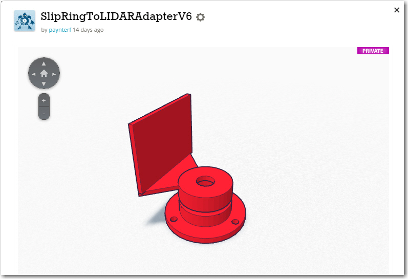
Original and 2nd versions of the LIDAR slip ring assembly mount
Once I was satisfied that the miniature motor, the tach wheel and tach sensor assembly, and the spinning LIDAR mount were all usable, I assembled the entire system and tested it using an Arduino test sketch.
After a few tests, and some adjustments to the tach sensor setup, I felt I had a workable spinning LIDAR setup, and was optimistic that I would have Wall-E ‘back on the road again’ within a few days, proudly going where no robot had gone before. However, I soon realized that a significant fly had appeared in the ointment – I wasn’t going to be able to accurately determine where the LIDAR was pointed – yikes! The problem was this; in order to tell Wall-E which way to move, I had to be able to map the surroundings with the LIDAR. In order to do that, I had to be able to associate a relative angle (i.e. 30 degrees to the right of Wall-E’s nose) with a distance measurement. Getting the distance was easy – just ask the LIDAR for a distance measurement. However, coming up with the relative angle was a problem, because all I really know is how fast the motor shaft is turning, and how long it has been since the index plug on the tach wheel was last ‘seen’. Ordinarily this information would be sufficient to calculate a relative angle, but in this case it was complicated by the fact that the LIDAR turntable is rotating at a different rate than the motor, due to the difference in pulley diameters – the drive ratio. For every 24mm diameter drive pulley rotation, the 26mm diameter LIDAR pulley only rotates 24/26 times, meaning that the LIDAR ‘falls behind’ more and more each rotation. So, in order to determine the current LIDAR pointing angle, I would have to know not only how long it has been since the last index plug sighting, but also how many times the drive pulley has rotated since the start of the run, and the exact relative positions of the drive pulley and the LIDAR at the start of the run. Even worse, the effect of any calculation errors (inaccurate pulley ratio, roundoff errors, etc) is cumulative, to the point where after a few dozen revolutions the angle calculation could be wildly inaccurate. And this all works only if the drive belt has never slipped at all during the entire run. Clearly this was not going to work in my very non-ideal universe :-(.
After obsessing over this issue for several days and nights, I finally came to the realization that there was only one real solution to this problem. The tach wheel and sensor had to be moved from the motor drive side of the drive belt to the LIDAR side. With the tach wheel/sensor on the LIDAR side, all of the above problems immediately and completely disappear – calculation of the LIDAR pointing angle becomes a simple matter of measuring the time since the last index plug detection, and calculation errors don’t accumulate. Each time the index plug is detected, the LIDAR’s pointing angle is known precisely; pointing angle calculation errors might accumulate during each rotation, but all errors are zeroed out at the next index plug detection. Moreover, the pointing angle calculation can be made arbitrarily accurate (to the limit of the Arduino’s computation capability and timer resolution) by using any per-revolution error term to adjust the time-to-angle conversion factor. As a bonus, the motor no longer has to be speed-controlled – I can run it open-loop and just measure the RPM using the tach wheel/sensor. As long as the motor speed doesn’t change significantly over multiple-revolution time scales, everything will still work.
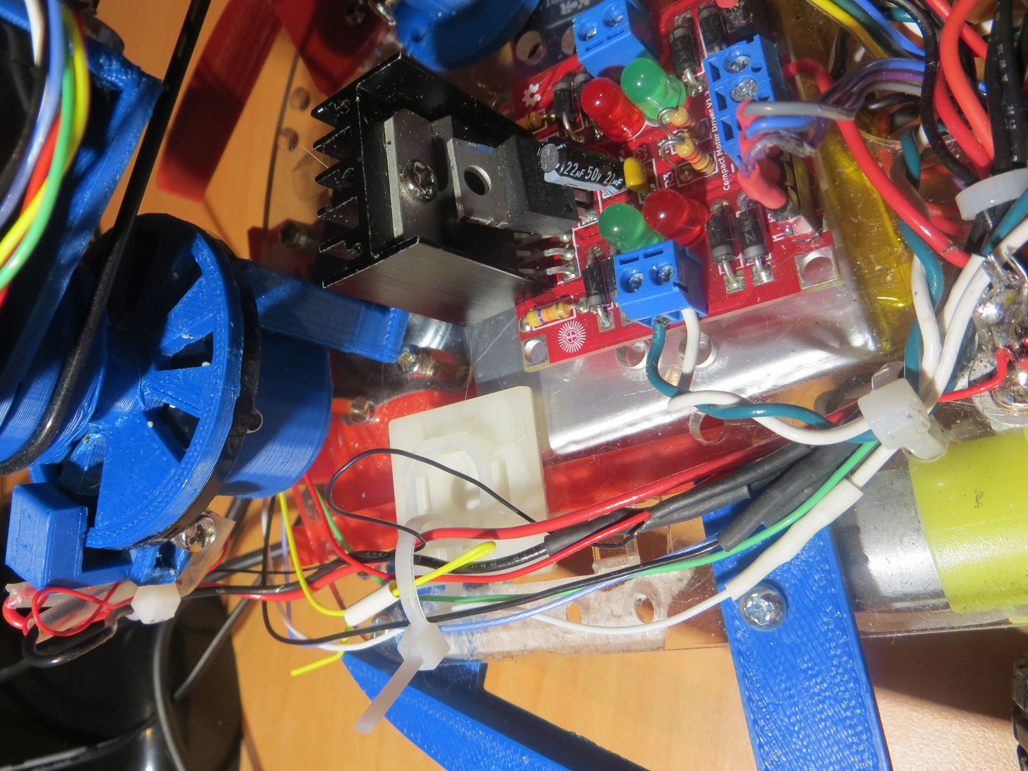
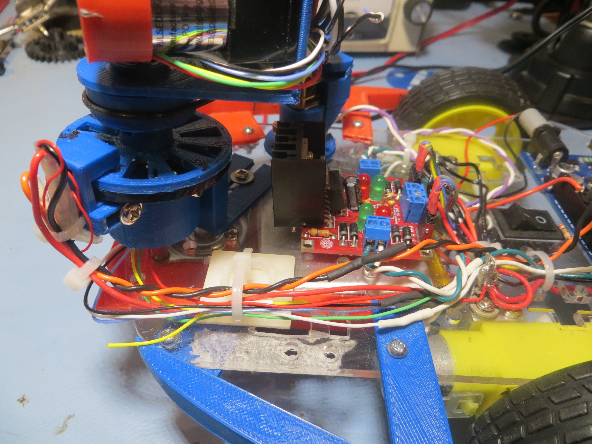
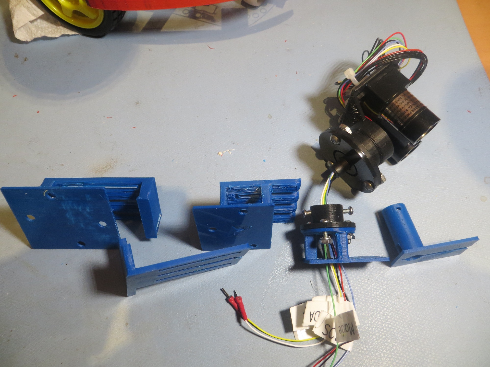
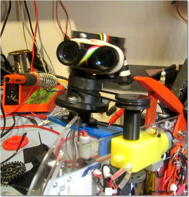
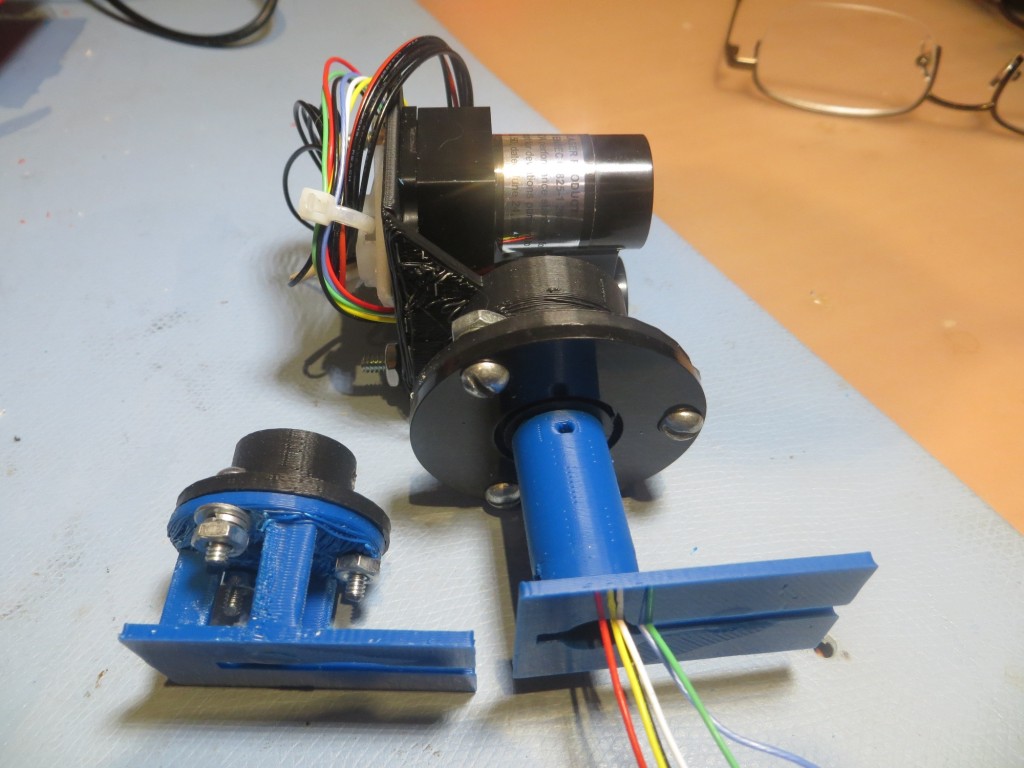
So, back to TinkerCad for major design change number 1,246,0025 :-). This time I decided to flip the 6-channel slip ring so the ‘big’ half was on the chassis side, and the ‘small’ half was on the LIDAR side, thereby allowing more room for the new tach wheel on the spinning side, and allowing for a smaller pulley diameter (meaning the LIDAR will rotate faster for a given motor speed). The result of the redesign is shown in the following photo.

Revised LIDAR and DC motor mounting scheme, with Tach wheel and sensor moved to LIDAR mount
In the above photo, note the tach sensor assembly is still on the motor mount (didn’t see any good reason to remove it. The ‘big’ (non-spinning) half of the slip ring module is mounted in a ‘cup’ and secured with two 6-32 set screws, and the tach wheel and LIDAR belt pulley is similarly mounted to the ‘small’ (spinning) half. The tach sensor assembly is a separate peice that attaches to the non-spinning ‘cup’ via a slotted bracket (not shown in the photo). The ‘big’ slip ring half is secured in the cup in such a way that one of the holes in the mounting flange (the black disk in the photo) lines up with the IR LED channel in the tach sensor assembly. The tach wheel spins just above the flange, making and breaking the LED/photo-diode circuit. Note also how the slip ring ‘cup’ was mounted on the ‘back’ side of the drive belt tension slide mount, allowing much better access to the slide mount friction screw. The right-angle LIDAR bracket was printed separately from the rest of the LIDAR assembly to get a ‘cleaner’ print, and then press-fit onto the pulley/tach wheel assembly via an appropriately sized hole in the LIDAR bracket. The following movie shows the whole thing in action
In the above movie, note the quality of the tach sensor signal; it is clamped to the voltage rails on both the upper and lower excursions, and the longer ‘high’ signal of the index plug is clearly visible at the far right of the oscilloscope screen.
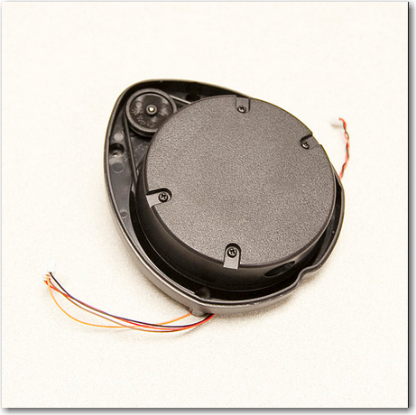
Details of the Tach Wheel:
Wall-E’s spinning LIDAR system features a tachometer wheel with an ‘index plug’, as shown below. Instead of a series of regularly spaced gaps, the gap in one section is missing, forming a triple-width ‘plug’ that allows me to detect the ‘index’ location. However, this means that instead of 20 equally spaced open-to-opaque or opaque-to-open transitions, there are only 18, as two of the transitions are missing. In addition, the LIDAR pointing angle isn’t as straightforward to calculate. If the trailing edge of the ‘index plug’ is taken as 0 degrees, then the next transition takes place at 18 degrees, then 36, 54, 72, 90, … to 306 degrees. However, after 306, the next transition isn’t 324 degrees – it is 360 (or 0) as the 324 and 342 degree transitions (shown in red in the diagram below) are missing. So, when assigning pointing angles to the interrupt number, I have to remember to multiply the interrupt index number (0 – 17) by 18 degrees (17*18 = 306). This also means that there is no ability to ‘see’ obstacles in the 54 degree arc from 306 to 360 degrees.
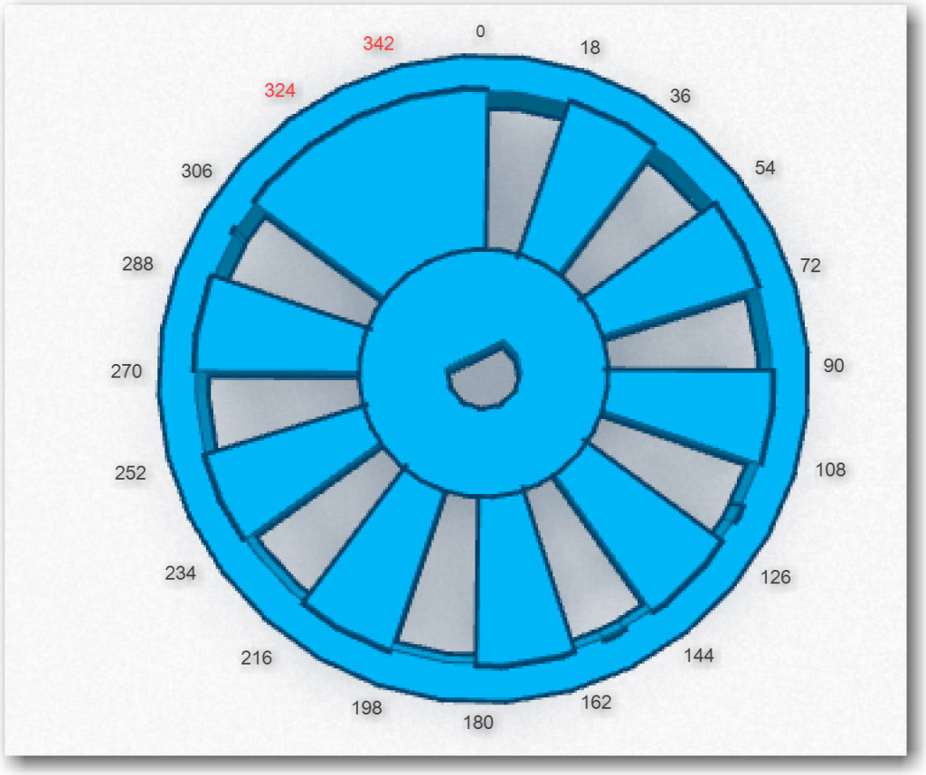
Diagram of the tach wheel for Wall-E’s spinning LIDAR system
Next Steps: Now that I have a LIDAR rotation system that works, the next step is to design, implement and test the program to acquire LIDAR distance data and accurately associate a distance measurement with a relative angle. With the new tach wheel/sensor arrangement, this should be relatively straightforward – but how to test? The LIDAR will be spinning at approximately 100 RPM, so it will be basically impossible to simply look at it and know where it is/was pointing when a particular measurement was taken, so how do I determine if the relative angle calculations are correct?
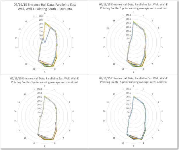
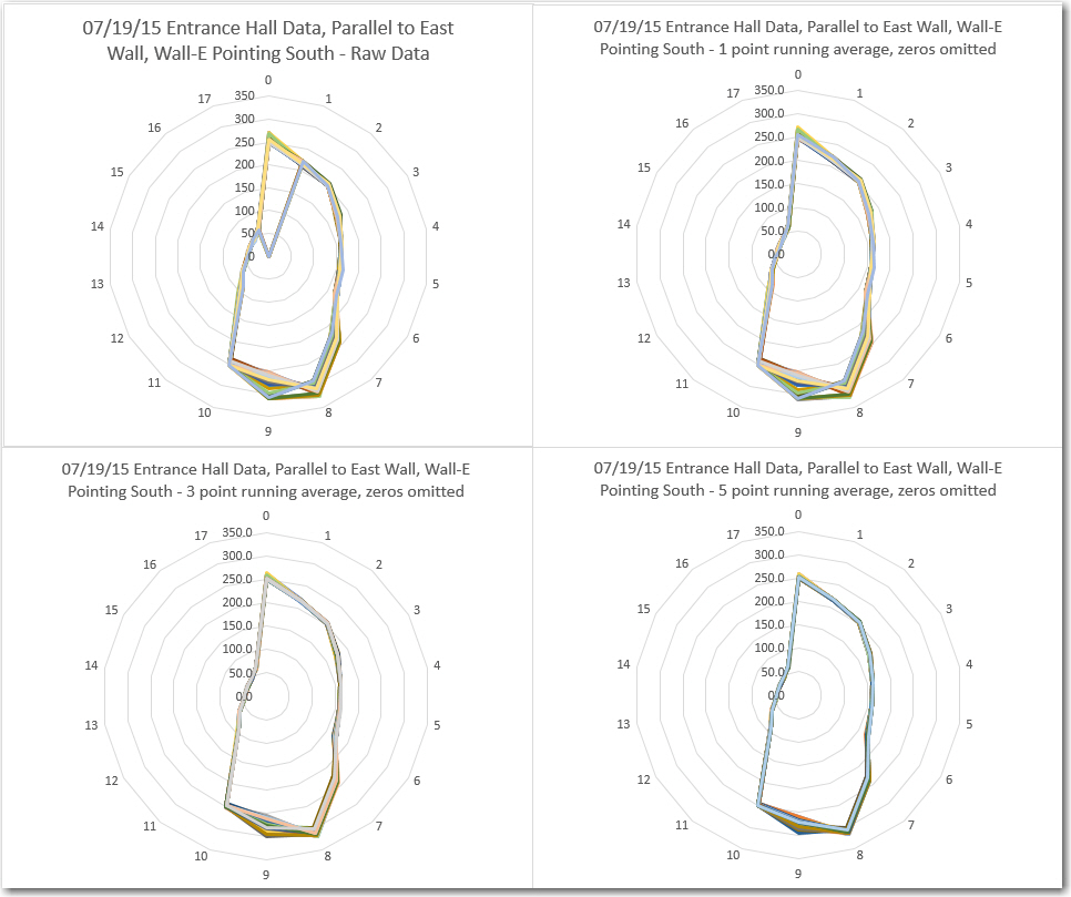
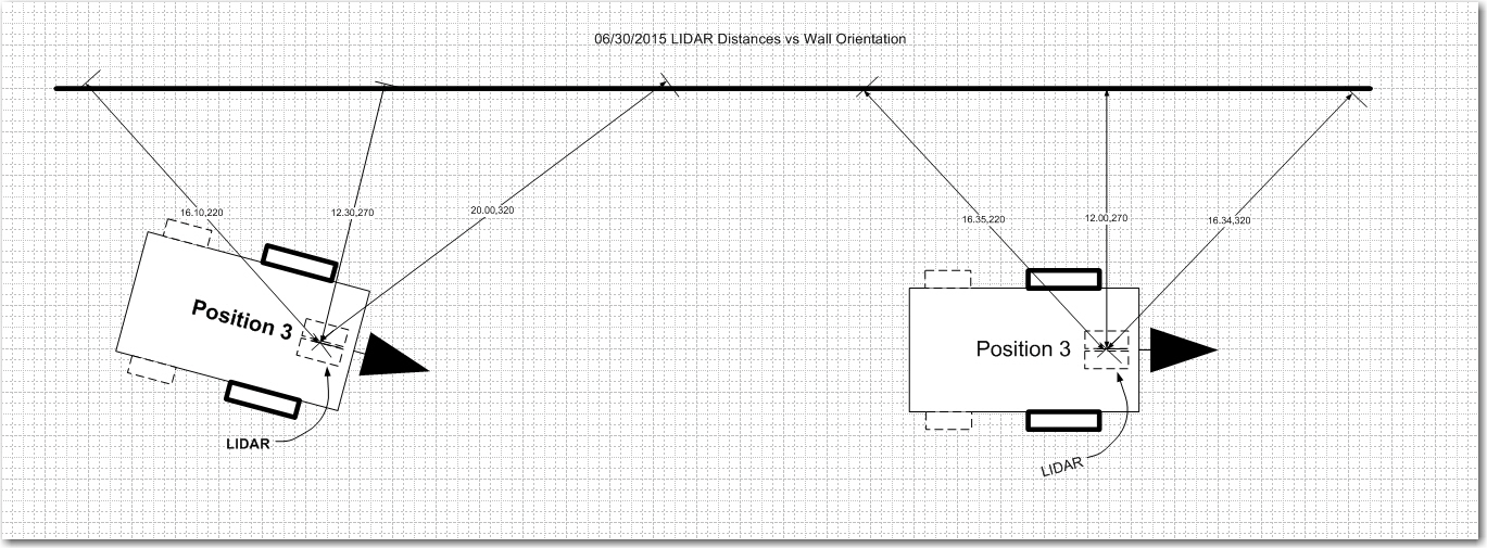
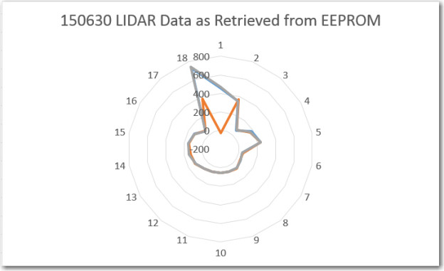
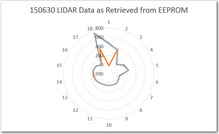
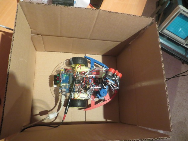
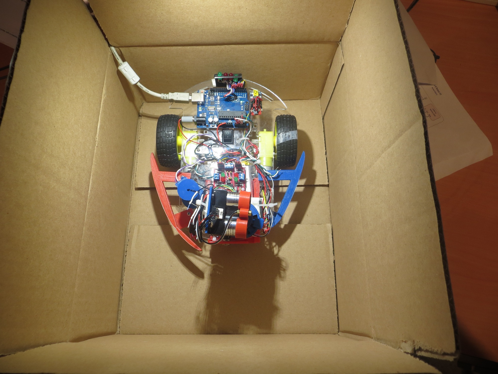
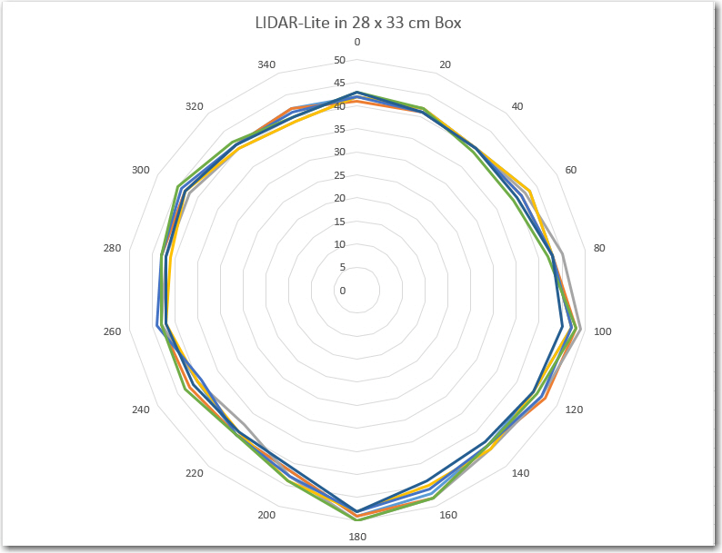
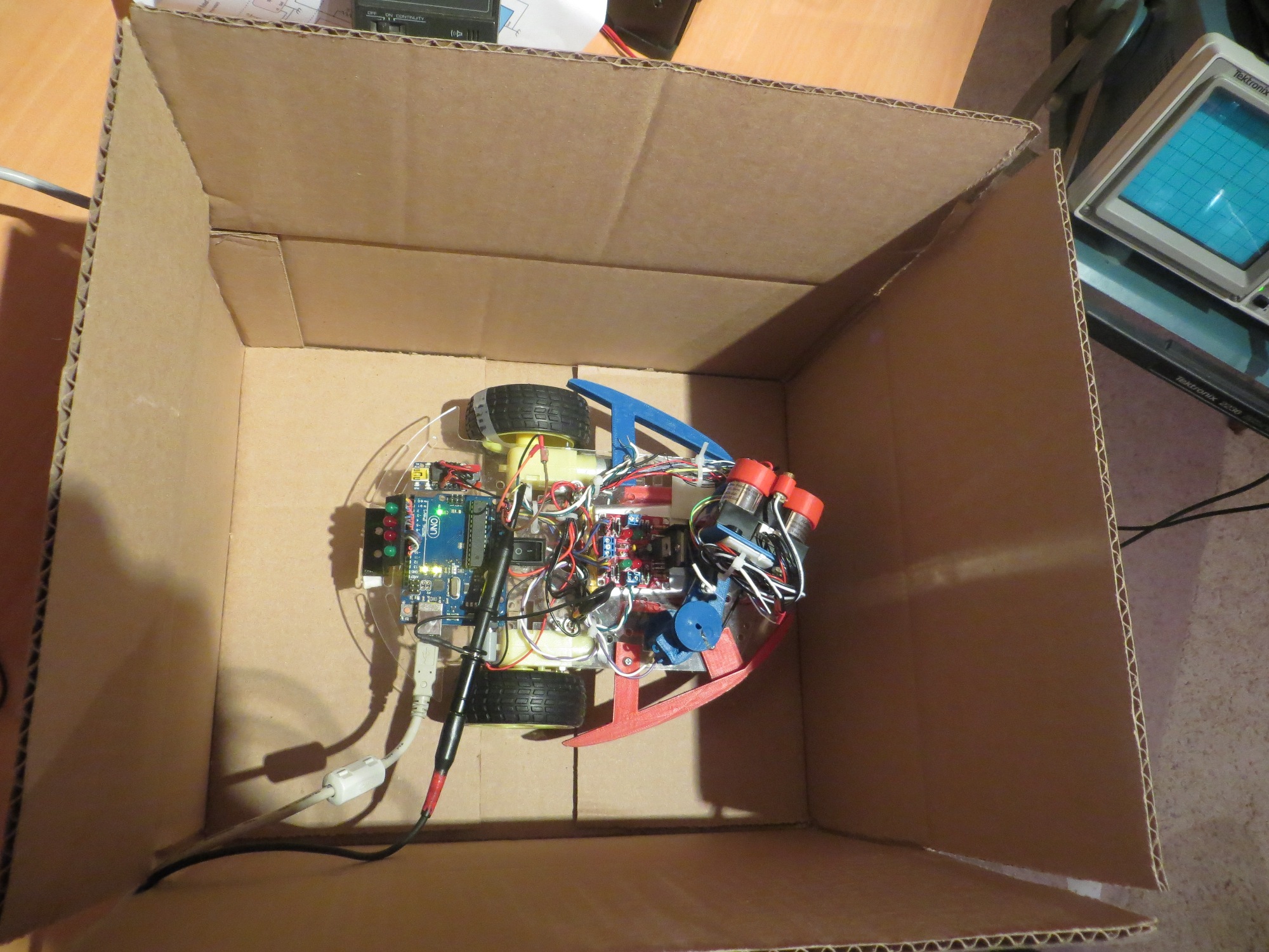
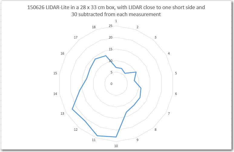
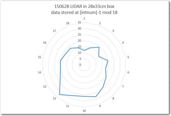
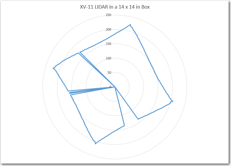
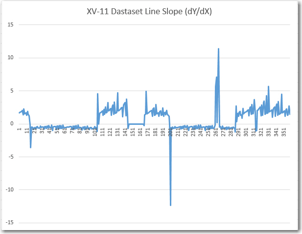
- I could put the whole think in a large cardboard box like I did with the XV-11 NEATO spinning LIDAR system (see ‘Fun with the NEATO XV-11 LIDAR module‘); If the (angle, distance) data pairs acquired accurately depict the walls of the container over multiple runs, that would go a long way toward convincing myself that the system is working correctly. I think that if the angle calculation was off, the lines plotted in one run wouldn’t line up with the ones from subsequent runs – in other words the walls of the box would blur or ‘creep’ as more data was acquired. I could also modify the box with a near-distance feature at a known relative angle to Wall-E’s nose, so it would be easy to tell if the LIDAR’s depiction of the feature was in the right orientation.
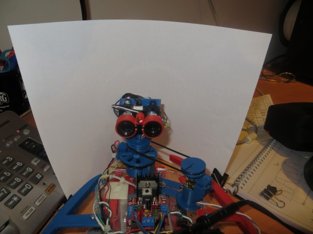
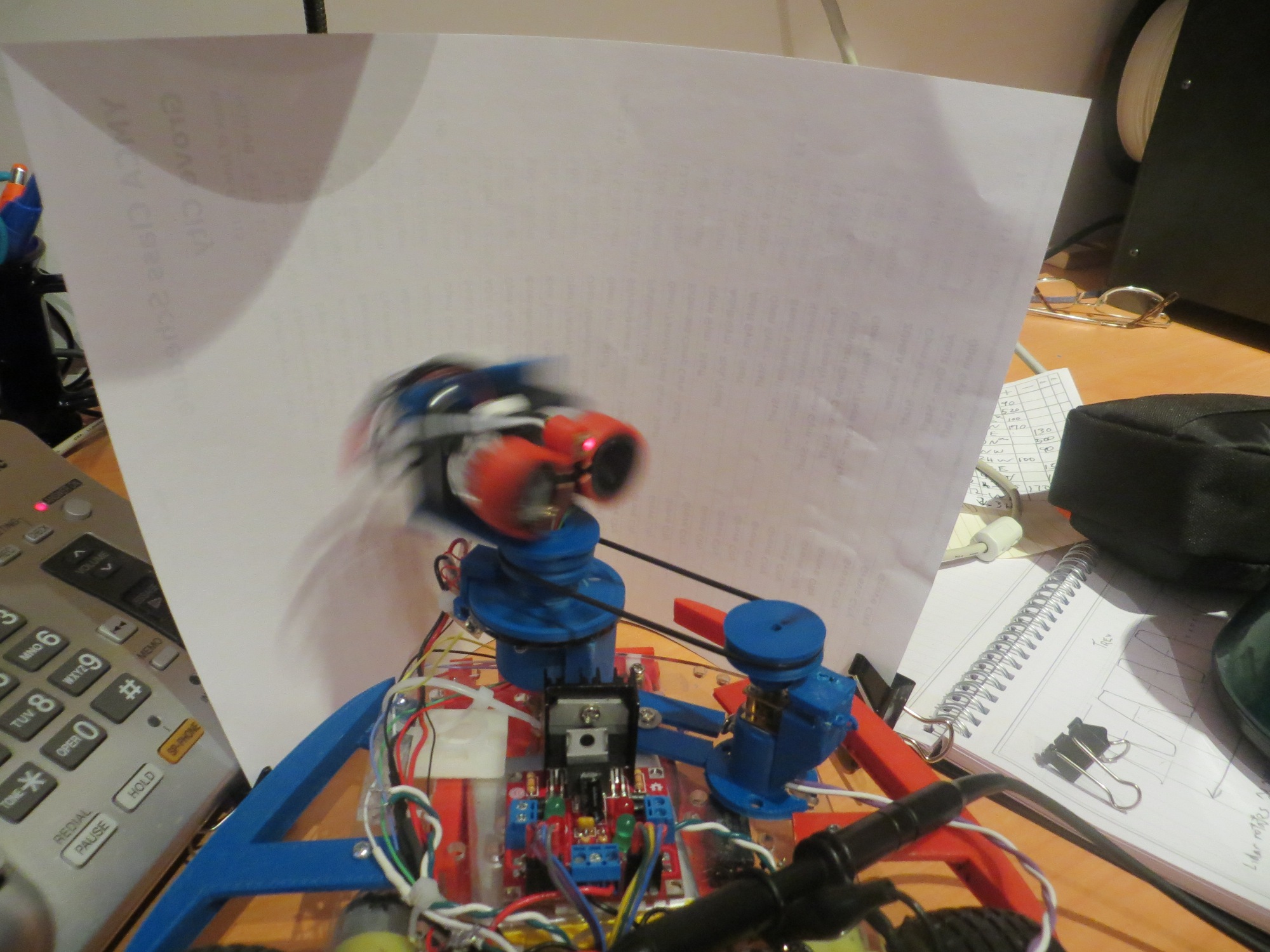
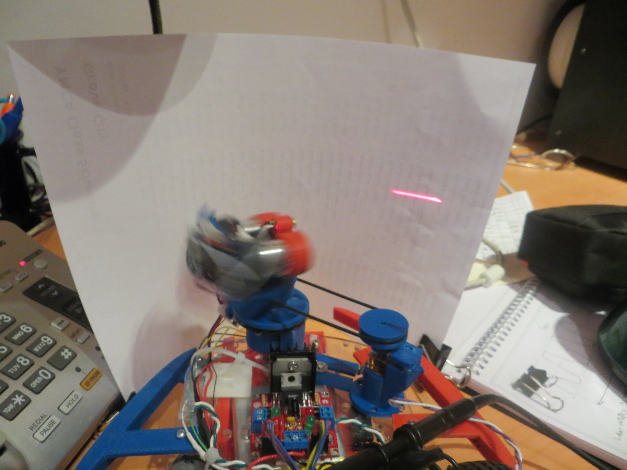
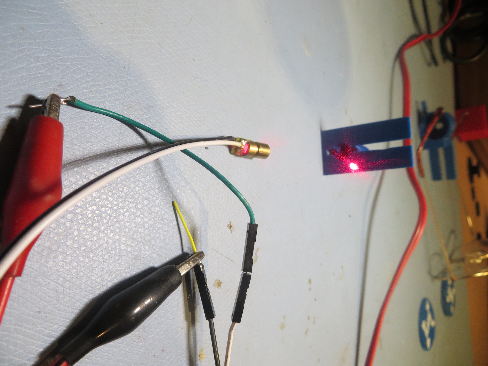
- I could mount a visible laser (similar to a common AV pointer) to the LIDAR so I could see where it is pointing. This would be a bit problematic, because this would simply paint a circle on the walls of the room as the LIDAR spins. In order to use a visible laser as a calibration device, I’d need to ‘blink’ it on and off in synchronism with the angle calculation algorithm so I could tell if the algorithm was operating correctly. For instance, if I calculated the required time delay (from the index plug detection time) for 0 degrees relative to the nose, and blinked the laser at that time, I should see a series of on/off dots directly in front of Wall-E’s nose. If the dots appear at a different angle but are stationary, then I have a constant error term somewhere. It they drift left or right, then I have a multiplicative factor error somewhere.
I think I’ll try both techniques; the box idea sounds good, but it may take a pretty large box to get good results (and I might even be better off using my entire office), and it might be difficult to really assess the accuracy of the system. I already have a visible laser diode, so implementing the second idea would only require mounting the laser diode on top of the LIDAR and using two of the 6 slip ring channels to control it. I have plenty of digital I/O lines available on the Arduino Uno, so that wouldn’t be a problem.
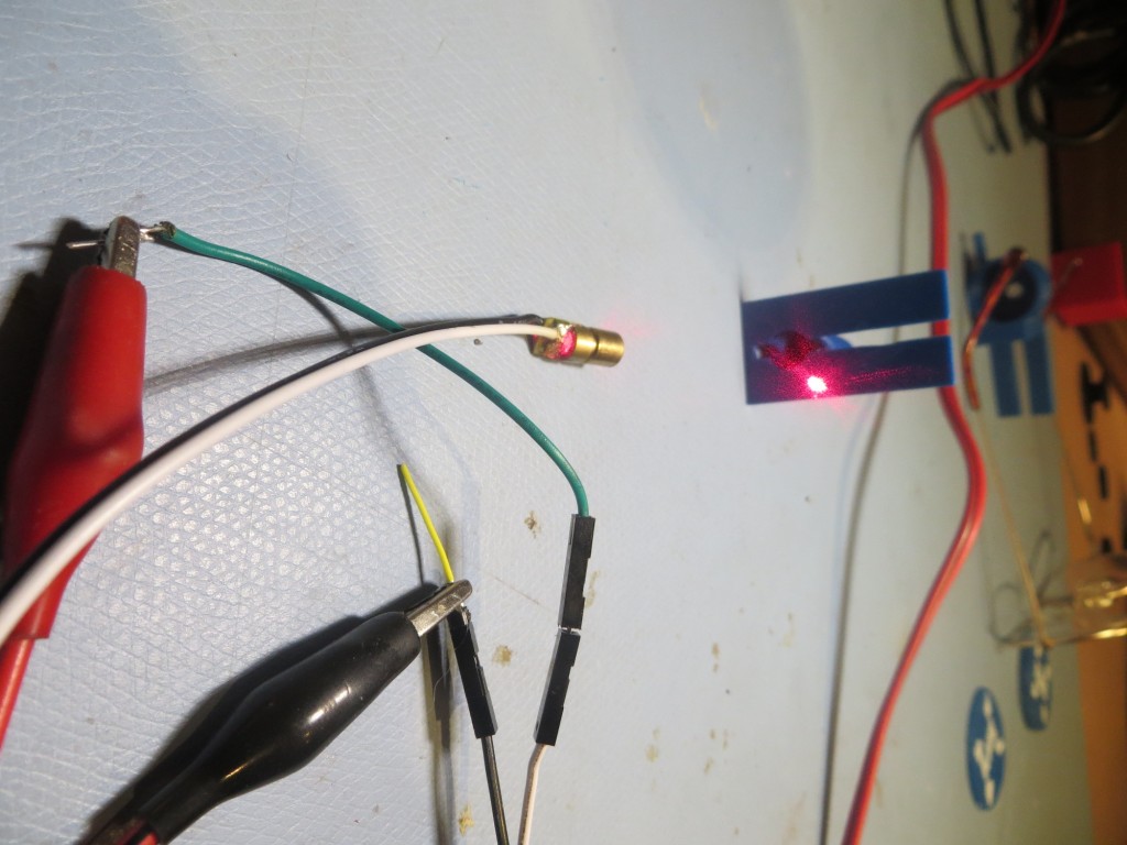
RobotGeek Laser, Item# ASM-RG-LASER available from Trossen Robotics (TrossenRobotics.com)
Stay tuned!
Frank