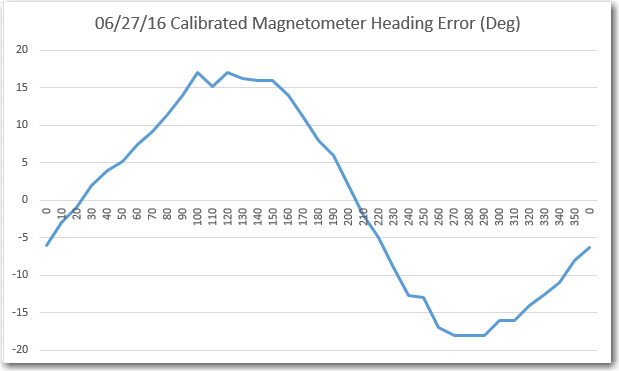
In my last episode of the Magnetometer Calibration Tool soap opera, I had a ‘working’ WPF application that could be used to generate a 3×3 calibration matrix and 3D center offset value for any magnetometer capable of producing 3D magnetometer values via a serial port. Although the tool worked, it had a couple of ‘minor’ deficiencies:
- My original Eyeshot-based tool sported a very nice set of 3D reference circles in both the ‘raw’ and ‘calibrated viewports. In the ‘raw’ view, the circle radii were equal to the average 3D distance of all point cloud points from the center, and in the ‘calibrated’ view the circle radii were exactly 1. This allowed the user to readily visualize any deviations from ideal in the ‘raw’ view, and the (hopefully positive) effect of the calibration algorithm. This feature was missing from the WPF-based tool, mainly because I couldn’t figure out how to do it :-(.
- The XAML and ‘code-behind’ associated with the project was a god-awful mess! I had tried lots and lots of different things while blindly stumbling toward a ‘mostly working’ solution, and there was a LOT of dead code and inappropriate structure still hanging around. In addition to being ugly, this state of affairs also reflected my (lack of) understanding of basic WPF/Helix Toolkit concepts, principles, and methods.
So, this post describes my attempts to rectify both of these problems. Happily, I can report that the first one (lack of switchable reference circles) has been completely solved, and the second one (god-awful mess and lack of understanding) has been at least partially rectified; I have a much better (although not complete by any means!) grasp of how XAML and ‘code-behind’ works together to produce the required visual effects.
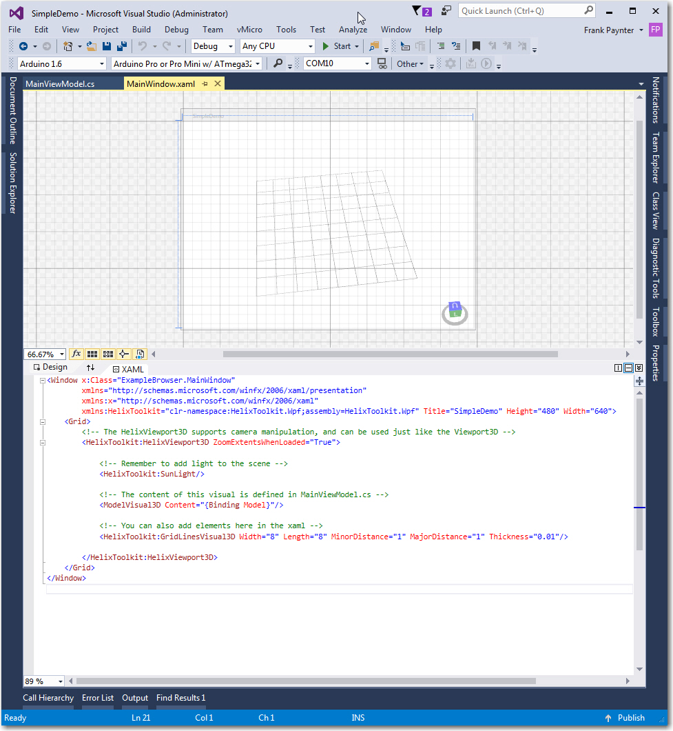
To achieve better understanding of the connection between the 3D viewport implemented in Helix Toolkit by the HelixViewport3D object, the XAML that describes the window’s layout, and the ‘code-behind’ C# code, I spent a lot of quality time working with and modifying the Helix Toolkit’s ‘Simple Demo’ app. The ‘Simple Demo’ program displays 3 box-like objects (with some spheres I added) on a grid, as shown below
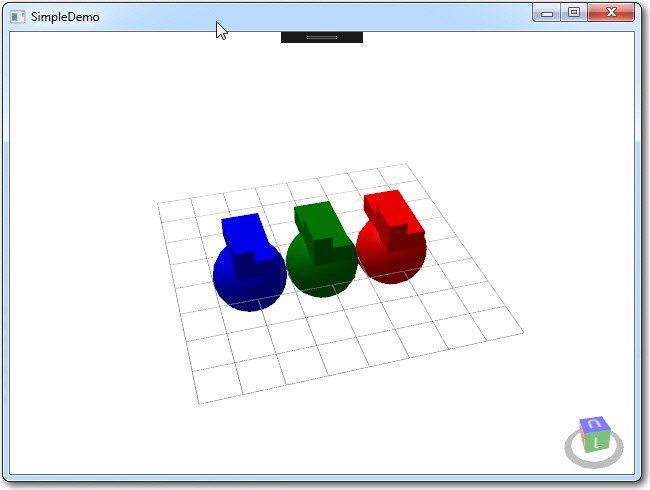
Simple Demo WPF/Helix Toolkit Application (spheres added by me)

Simple Demo XAML View – no changes from original
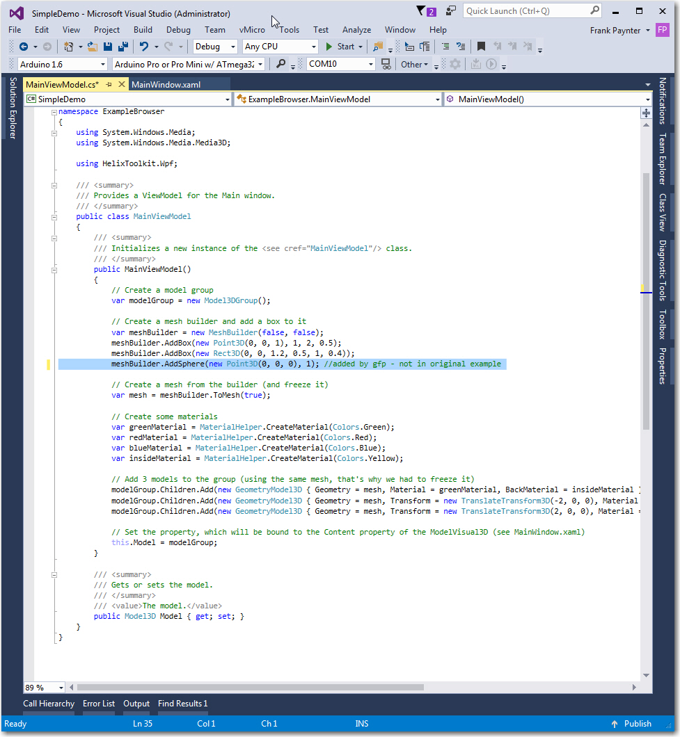
Simple Demo ‘Code-behind’, with my addition highlighted
My aim in going back to the ‘Simple Demo’ was to avoid the distraction of my more complex window layout (2 separate HelixViewport3D windows and lots of other controls) and the associated C#/.NET code so I could concentrate on one simple task – how to implement a set of 3D reference circles that can be switched on/off via a windows control (a checkbox in my case). After trying a lot of different things, and with some clues garnered from the Helix Toolkit forum, I settled on the TubeVisual3D object to construct the circles, as shown in the following screenshots. I used an empirically determined ‘thickness factor’ of 0.05*Radius for the ‘Diameter’ property to get the ‘thick circular line’ effect I wanted.
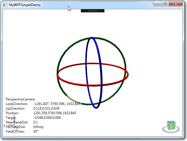
Simple Demo modified to implement TubeVisual3D objects. The original box/sphere stuff is still there, just too small to see
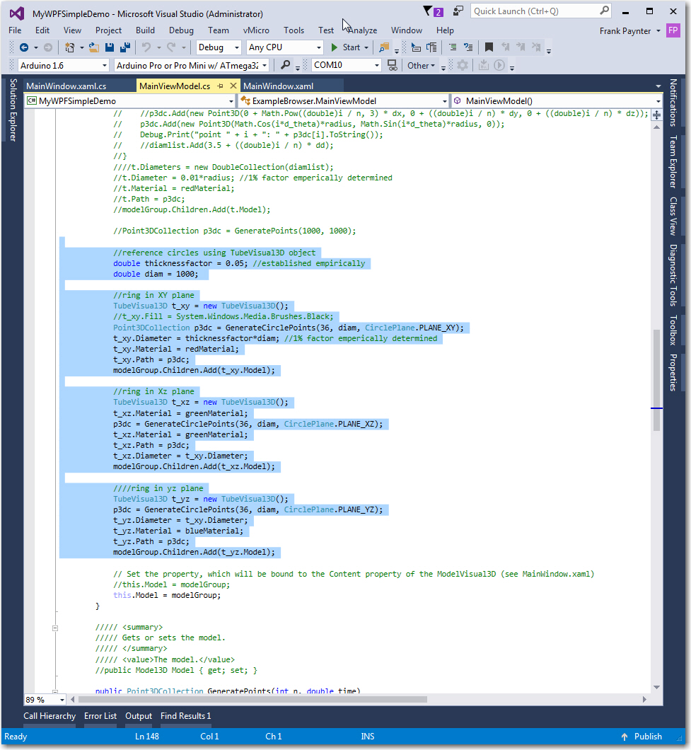
MyWPFSimpleDemo ‘code-behind’, with TubeVisual3D implementation code highlighted. Note all the ‘dead’ code where I tried to use the EllipsoidVisual3D model for this task.
Next, I had to figure out a way of switching the reference circle display on and off using a windows control of some sort, and this turned out to be frustratingly difficult. It was easy to get the circles to show up on program startup – i.e. with model construction and the connection to the viewport established in the constructor(s), but I could not figure out a way of doing the same thing after the program was already running. I knew this had to be easy – but damned if I could figure it out! Moreover, after hours of searching the blogosphere, I couldn’t find anything more than a few hints about how to do it. What I did find was a lot of WPF beginners like me with the same problem but no solutions – RATS!!
Finally I twigged to the fundamental concept of WPF 3D visualization – the connection between a WPF viewport (the 2D representation of the desired 3D model) and the ‘code-behind’ code that actually represents the 3D entities to be displayed must be defined at program startup, via the following constructs:
- In the XAML, a line like ‘<ModelVisual3D Content=”{Binding Model}”/>, where Model is the name of a Model3D property declared in the ‘code-behind’ file (MainViewModel.cs in my case)
- In MainWindow.xaml.cs, a line like ‘this.DataContext = mainviewmodel’, where mainviewmodel is declared with ‘public MainViewModel mainviewmodel = new MainViewModel();’
- In MainViewModel.cs, a line like ‘ public Model3D Model { get; set; }’, and in the class constructor, ‘Model = new Model3DGroup();’
- in MainViewModel.cs, the line ‘var modelGroup = new Model3DGroup();’ at the top of the model creation section to create a temporary Model3DGroup object, and the line ‘ this.Model = modelGroup;’ at the bottom of the model construction code. This line sets the Model property contents to the contents of the temporary ‘modelGroup‘ object
So, the ‘MainViewModel’ class is connected to the Windows window class in MainWindow.xaml.cs, and the 3D model described in the MainViewModel class is connected to the 3D viewport via the Model Model3DGroup object. This is all done at initial object construction, in the various class constructors. There are still some parts of this that I do not understand, but I think I have it mostly correct.
The important concept that I was missing is the above connections have been made at program startup and cannot (AFAICT) be changed once the program starts, but the contents of the temporary Model3DGroup object (i.e. the ‘Children’ objects in the model group) can be changed, and the new contents will be reflected in the viewport when it is next updated. Once I understood this concept, the rest, as they say, “was history”. I implemented a simple control handler that cleared the contents of the temporary Model3DGroup object modelGroup and regenerated it (or not, depending on the state of the ‘Show Ref Circles’ checkbox). Simple and straightforward, once I knew the secret!
So this ‘aha’ moment allowed me to implement the switchable reference circles in my Magnetometer calibration tool and check off the first of the deficiencies noted at the start of this post. The new reference circle magic is shown in the following screenshots.
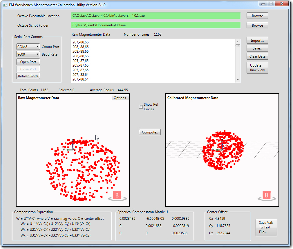
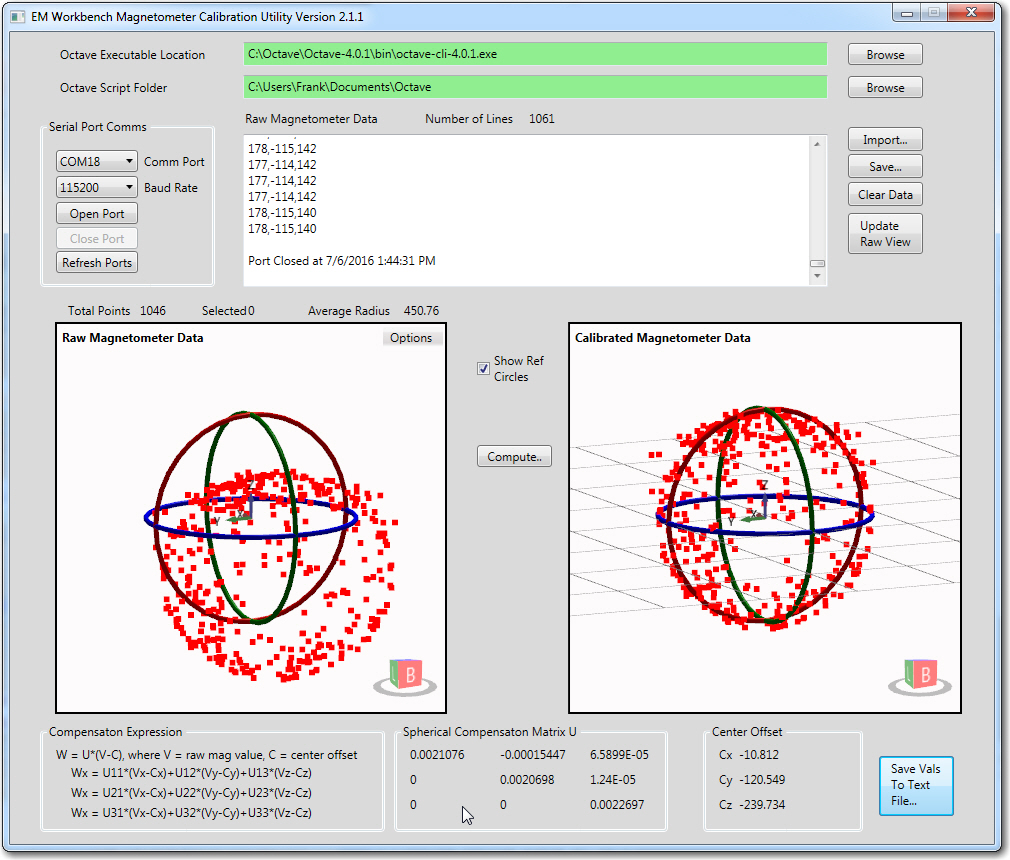
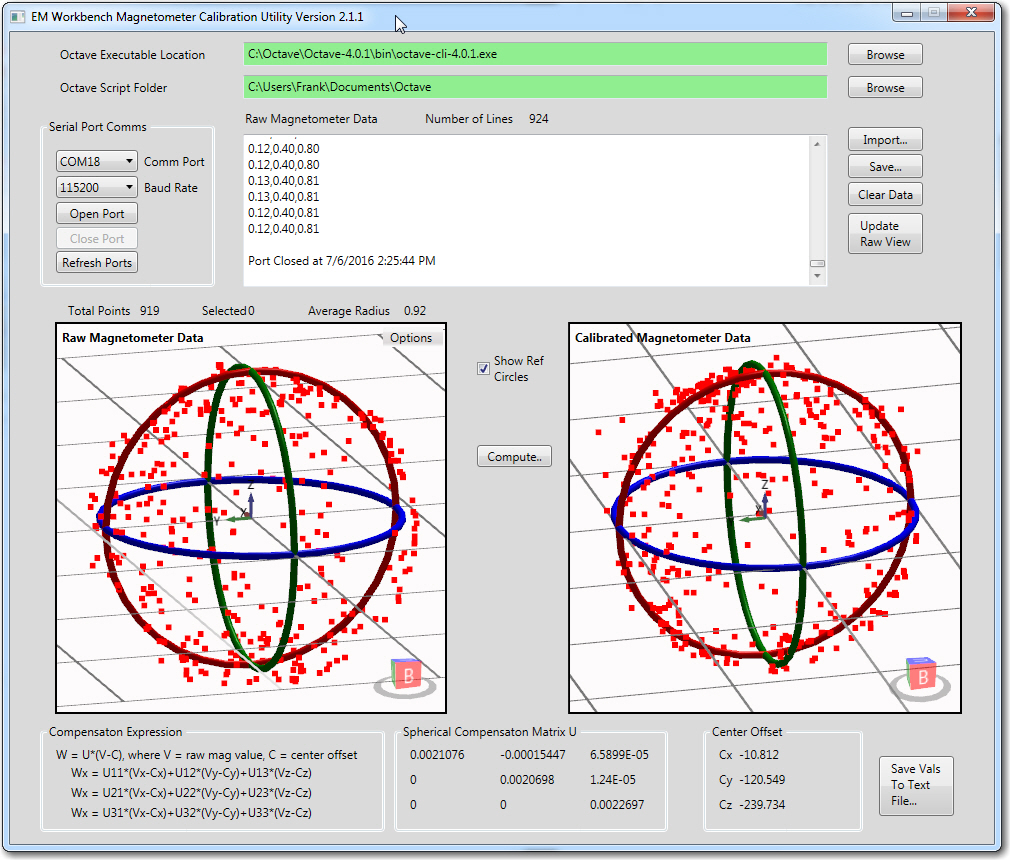
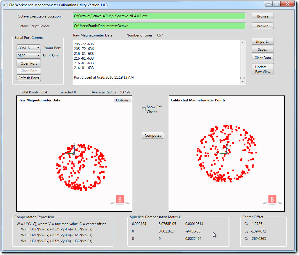
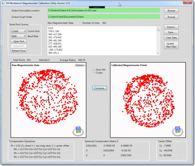
Raw and calibrated magnetometer data. Calculated average radius of the raw data is about 444 units, and the assumed average radius of the calibrated data is close to 1 unit
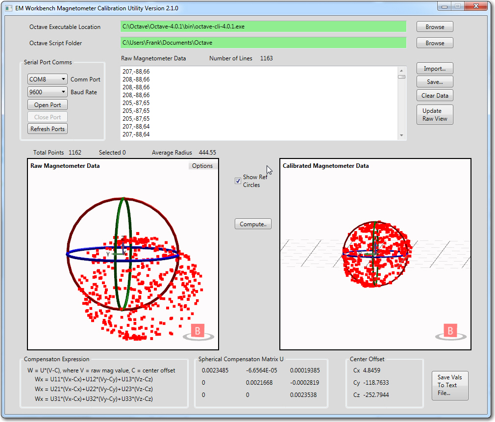
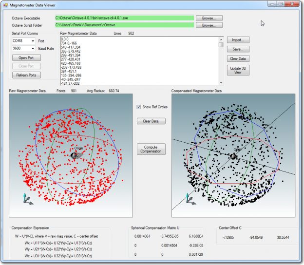
Raw and calibrated magnetometer data, with reference circles shown. The radius of the ‘raw’ circles is equal to the calculated average radius of about 444 units, and the assumed average radius of the calibrated circles is exactly 1 unit
The reference circles make it easy to see how the calibration process affects the data. In the ‘raw’ view, it is apparent that the data is significantly offset from center, but still reasonably spherical. In the calibrated view, it is easy to see that the calibration process centers the data, removes most of the non-sphericity, and scales everything to very nearly 1 unit – nice!
Now for addressing the second of the two major deficiencies noted at the start of this post, namely “The XAML and ‘code-behind’ associated with the project was a god-awful mess! “.
With my current understanding of a typical WPF-based application, I believe the application architecture consist of three parts – the XAML code (in MainWindow.xaml) that describes the window layout, the ‘MainWindow’ class (in MainWindow.cs) that contains the interaction logic with the main window, and a class or classes that generate the 3D models to be rendered in the main window. For my magnetometer calibration tool I created two 3D model generation classes – ViewportGeometryModel and RawViewModel. The ViewportGeometry class is the base class for RawViewModel, and handles generation of the three orthogonal TubeVisual3D ‘circles. The ViewportGeometryModel class is instantiated directly (as ‘calmodel’ in the code) and connected to the main window’s ‘vp_cal’ HelixViewport3D window via it’s ‘GeometryModel’ Model3D property, and the derived class RawViewModel (instantiated in the code as ‘rawmodel’) is similarly connected to the main window’s ‘vp_raw’ HelixViewport3D window via the same ‘GeometryModel’ Model3D property (different object instantiation, same property name).
The ViewportGeometryModel class has one main function, and some helper stuff. The main function is ‘DrawRefCircles(HelixViewport3D viewport, double radius = 1, bool bEnable = false)’. This function is called from MainWindow.xaml.cs as follows:
1 2 3 4 5 6 7 8 9 10 11 12 13 14 15 16 17 18 19 20 |
public MainWindow() { InitializeComponent(); //connect raw/cal viewports to their respective geometry model classes rawmodel = new RawViewModel(vp_raw, this); //ctor creates an empty 3D model & loads it into the raw view's 'GeometryModel' property calmodel = new ViewportGeometryModel(vp_cal, this);//ctor creates an empty 3D model & loads it into the calibrated view's 'GeometryModel' property vp_raw.DataContext = rawmodel; //this tells vp_raw to use the 'rawmodel' object's 'GeometryModel' property vp_cal.DataContext = calmodel; //this tells vp_raw to use the 'calmodel' object's 'GeometryModel' property ..... (other stuff) } private void chk_RefCircles_Click(object sender, RoutedEventArgs e) { System.Windows.Controls.CheckBox cbx = (System.Windows.Controls.CheckBox)sender; bool check = cbx.IsChecked ?? false; //'??' needed in case cbx is null <em><strong>rawmodel.DrawRefCircles(vp_raw, rawmodel.GetRawAvgRadius(), check);</strong> <strong>calmodel.DrawRefCircles(vp_raw, 1, check);</strong></em> } |
The ‘DrawRefCircles()’ function creates a new ModelGroup3D object if necessary, and optionally fills it with three TubeVisual3D objects of the desired radius and thickness, as shown below
1 2 3 4 5 6 7 8 9 10 11 12 13 14 15 16 17 18 19 20 21 22 23 24 25 26 27 28 29 30 31 32 33 34 35 36 37 38 39 40 41 42 43 44 45 46 47 48 49 50 51 52 53 54 |
public void DrawRefCircles(HelixViewport3D viewport, double radius = 1, bool bEnable = false) { //// Create a model group if (modelGroup == null) { modelGroup = new Model3DGroup();// Create an empty model group if necessary } else //already exists - remove all children so we can start over { modelGroup.Children.Clear(); } if (bEnable) //if checkbox state is 'checked', create the ref circle objects { // Create the materials (colors) we will need var greenMaterial = MaterialHelper.CreateMaterial(Colors.Green); var redMaterial = MaterialHelper.CreateMaterial(Colors.Red); var blueMaterial = MaterialHelper.CreateMaterial(Colors.Blue); //create reference circles using TubeVisual3D objects //probably should do this using transforms, but don't know how :-( double thicknessfactor = 0.05; //established empirically //ring in XY plane TubeVisual3D t_xy = new TubeVisual3D(); //t_xy.Fill = System.Windows.Media.Brushes.Black; Point3DCollection p3dc = GenerateCirclePoints(36, radius, CirclePlane.PLANE_XY); t_xy.Diameter = thicknessfactor * radius; //1% factor emperically determined t_xy.Material = blueMaterial; //to match viewport coord sys colors t_xy.Path = p3dc; modelGroup.Children.Add(t_xy.Model); //ring in Xz plane TubeVisual3D t_xz = new TubeVisual3D(); t_xz.Material = greenMaterial; p3dc = GenerateCirclePoints(36, radius, CirclePlane.PLANE_XZ); t_xz.Material = greenMaterial; //to match viewport coord sys colors t_xz.Path = p3dc; t_xz.Diameter = t_xy.Diameter; modelGroup.Children.Add(t_xz.Model); ////ring in yz plane TubeVisual3D t_yz = new TubeVisual3D(); p3dc = GenerateCirclePoints(36, radius, CirclePlane.PLANE_YZ); t_yz.Diameter = t_xy.Diameter; t_yz.Material = redMaterial; //to match viewport coord sys colors t_yz.Path = p3dc; modelGroup.Children.Add(t_yz.Model); } // GeometryModel is bound to HelixViewport3D with the line // in MainWindow.xaml) GeometryModel = modelGroup; } |
The last line in the above function is ‘GeometryModel = modelGroup;’, where ‘GeometryModel’ is declared in the ViewGeometryModel class as
|
|
public Model3D GeometryModel { get; set; } //this is bound to the viewport |
and bound to the appropriate HelixViewport3D window via

Line in MainWindow.xaml that binds the HelixViewport3D to the ‘GeometryModel’ Model 3D property of the ViewportGeometryModel class (and/or its derived class RawViewModel). The line shown here is for the raw viewport, and there is an identical one in the calibrated viewport section.
Now, instead of a mishmash spaghetti factory, the program is a lot more organized, modular, and cohesive (or at least I think so!). As the following screenshot shows, there are only a few classes, and each class does a single thing. Mission accomplished!
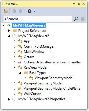
Magnetometer calibration tool class diagram. Note that the RawViewModel is a derived class from VieportGeometryModel. The ViewportGeometryModel.CirclePlane ‘class is an Enum
Other Stuff:
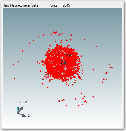
This entire post has been a description of how I figured out the connections between a WPF-based windowed application with two HelixViewport3D 3D viewports (and lots of other controls) and the XAML/code-behind elements that generate the 3D models to be rendered. In particular it has been a description of the ‘reference circle’ feature for both the ‘raw’ and ‘calibrated’ views. However, these circles are really only a small part of the overall magnetometer calibration tool; a much bigger part of the 3D view are the point-clouds in both the raw and calibrated views that depict the actual 3D magnetometer values acquired from the magnetometer being calibrated, before and after calibration. I didn’t say anything about these point-cloud collections, because I had them working long before I started the ‘how can I display these damned reference circles’ odyssey. However, I thought it might be useful to point out (no pun intended) some interesting tidbits about the point-cloud implementation.
- I implemented the point-cloud using the Helix Toolkit’s PointsVisual3D and Point3DCollection objects. Note that the PointsVisual3D object is derived from ScreenSpaceVisual3D which is derived from RenderingModelVisual3D instead of a geometry object like TubeVisual3D which is derived from ExtrudedVisual3D, which in turn is derived from MeshElement3D. These are very different inheritance chains. A PointsVisual3D object can be added directly to a HelixViewport3D object’s Children collection, and doesn’t need a light for rendering! I can’t tell you how much agony this caused me, as I just couldn’t understand why other objects added via the ModelGroup chain either didn’t render at all, or rendered as flat black objects. Fortunately for me, the ‘SimpleDemo’ app did have light already defined, so things displayed normally (it still took me a while to figure out that I had to add a light to my MagCal app, even though the point-cloud displayed fine).
- Points in a point-cloud collection don’t support a ‘selected’ property, so I had to roll my own selection facility. I did this by handling the mouse-down event, and manually checking the distance of each point in the collection from the mouse-down point. If I found a point(s) close enough, I manually moved the point from the ‘normal’ point-cloud to a ‘selected’ point-cloud, which I rendered slightly larger and with a different color. If a point became ‘unselected’, I manually moved it back into the ‘normal’ point-cloud object. A bit clunky, but it worked.
All of the source code, and a ZIP file containing everything (except Octave) needed to run the Magnetometer Calibration app is available at my GitHub site – https://github.com/paynterf/MagCalTool
Frank