Posted 01 July 2017
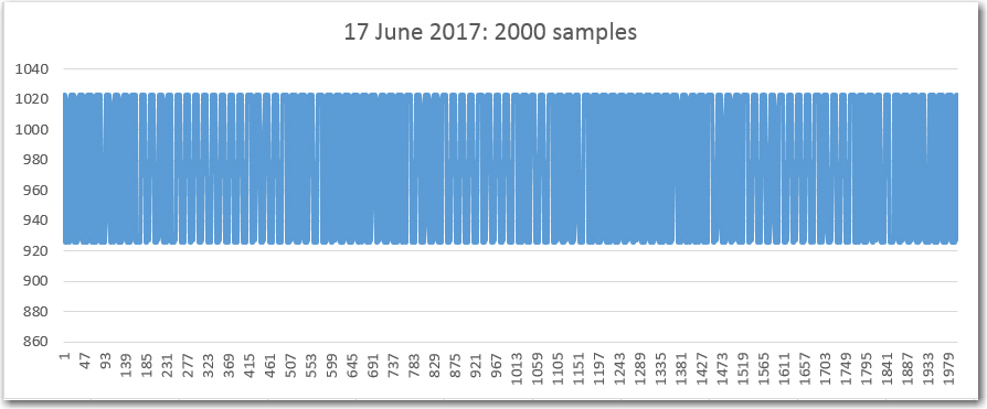
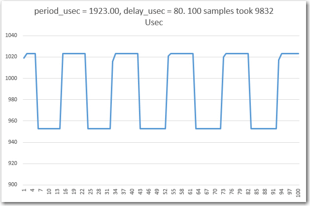
I went down a bit of a rabbit-hole between my last post on this subject and today. I was attempting to run down the problems with my IR demodulation code when I discovered that the basic rate at which the demodulator captured samples was off by a factor of 5 or so – yikes!! Instead of 20 samples per cycle, I was seeing more like 100, as shown below.
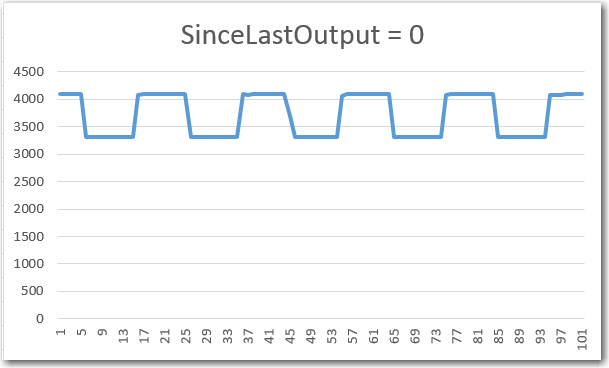
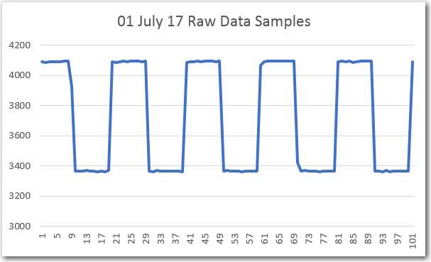
Raw data capture using ‘sinceLastOutput = 0’ in the first demodulation step
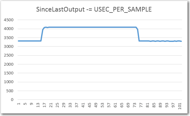
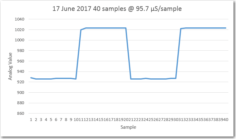
Raw data capture using ‘sinceLastOutput -= USEC_PER_SAMPLE’ in the first demodulation step
As you might expect, this development threw me for a bit of a loop – as the change from ‘sinceLastOutput = 0’ to ‘sinceLastOutput -= USEC_PER_SAMPLE’ was instrumental (or at least so I thought) to getting the transmit and receive frequencies matched more accurately. So, now I had to go chase down yet another tangential problem – what I refer to as ‘going down a rabbit hole’. The only saving grace in all this is that, as a twice-retired engineer, I have no deadlines! 😉
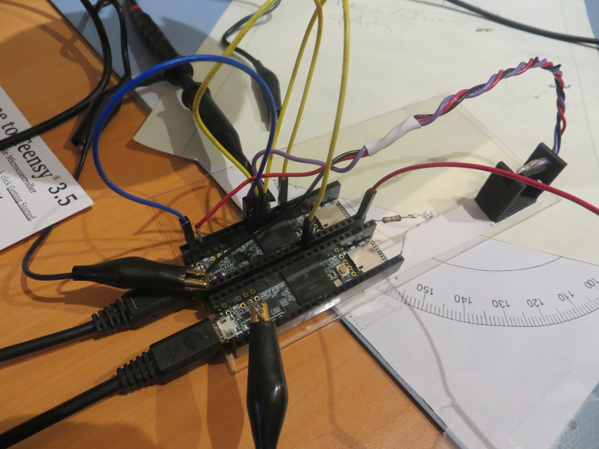
To resolve this problem, I wound up creating an entirely new test program to isolate the issue, with just the following lines in the loop() function:
|
1 2 3 4 5 6 7 8 9 10 11 12 13 14 15 16 17 18 19 20 |
void loop() { //this runs every 95.7uSec if (sinceLastOutput > USEC_PER_SAMPLE) { //sinceLastOutput = 0; sinceLastOutput -= USEC_PER_SAMPLE; //start of timing pulse digitalWrite(OUTPUT_PIN, HIGH); // Step1: Collect a 1/4 cycle group of samples and sum them into a single value // this section executes each USEC_PER_SAMPLE period int samp = adc->analogRead(SENSOR_PIN); Serial.print(sample_count); Serial.print("\t"); Serial.println(samp); sample_count++; //checked in step 6 to see if data capture is complete digitalWrite(OUTPUT_PIN, LOW); }//if (sinceLastOutput > 95.7) }//loop |
With the ‘sinceLastOutput -= USEC_PER_SAMPLE’ line active, I got about 100 samples/cycle. With this line commented out and the ‘sinceLastOutput = 0’ line active, I got the normal 20 samples/cycle, with nothing else being changed.
Once I was sure the test program was consistently producing the anomalous results I had noticed in the complete program, I posted this issue to the PJRC Forum, so I could get some help from the experts. I knew it was something I was doing wrong – I just didn’t know what!
Within a few hours I had received several responses, and the one that hit the bullseye was the one correctly identifying a subtlety with the the ‘-=’ elapsedMicros() usage format. When this format is used, the accompanying ‘elapsedMicros’ variable must be initialized in the setup() code; otherwise it will be some arbitrary (and possibly quite large) value when the loop() function is first entered. This will cause the ‘if’ statement to trigger repeatedly until the ‘-=’ line eventually reduces the variable to a value below USEC_PER_SAMPLE, at which point it will start behaving as expected. This odd behavior never happens with the ‘=0’ usage, as the variable is initialized on the first pass through the ‘if’ statement. Sure enough, when I added a line at the bottom of my setup() function to set the ‘sinceLastOutput’ variable to zero, my little test program immediately stopped mis-behaving.
Well, this little side-journey only cost me a couple of days, and a few more white hairs (oh, wait – my hair is already completely white – no problem!) Back to my regularly scheduled program…
Frequency Matching:
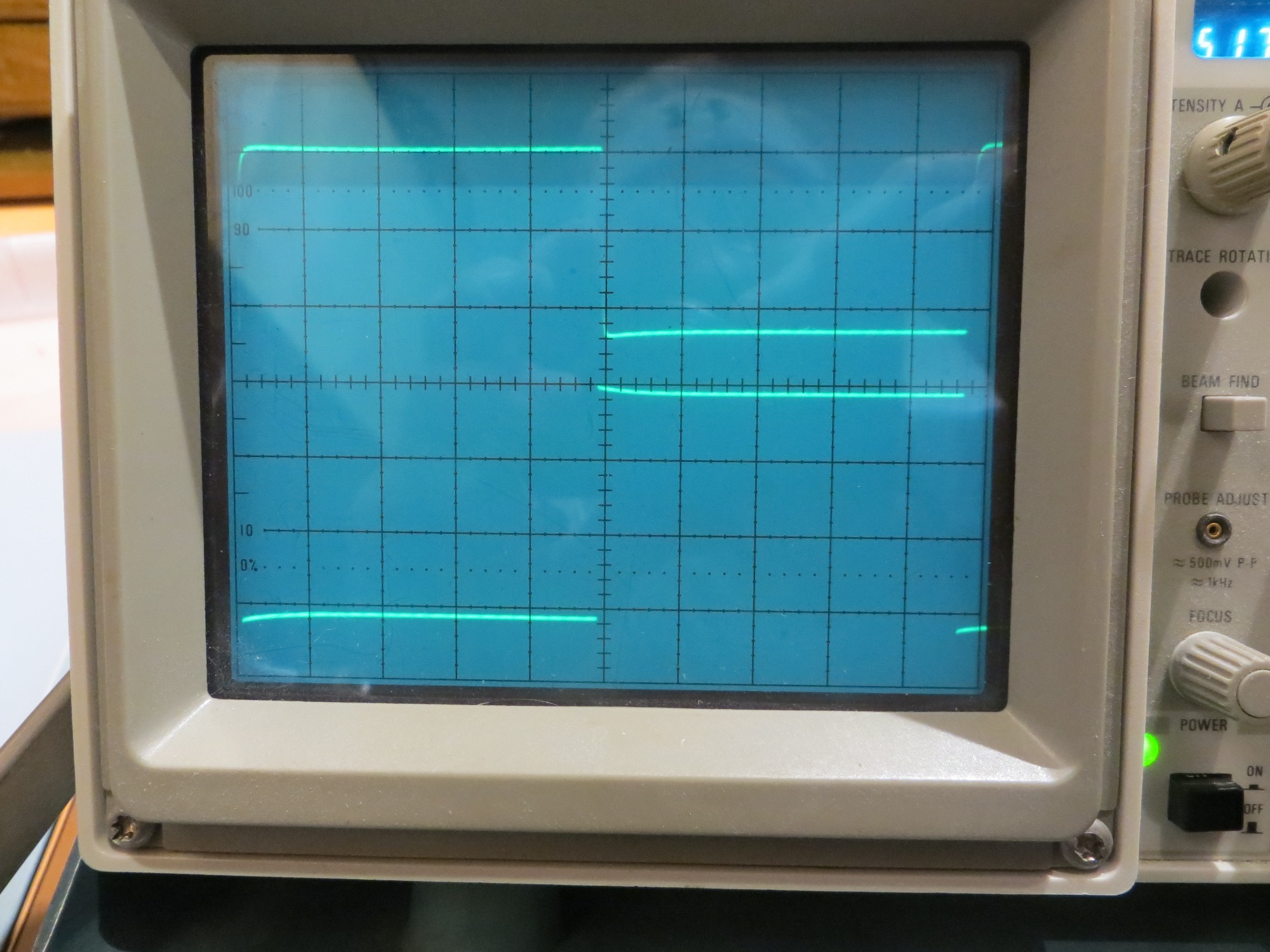
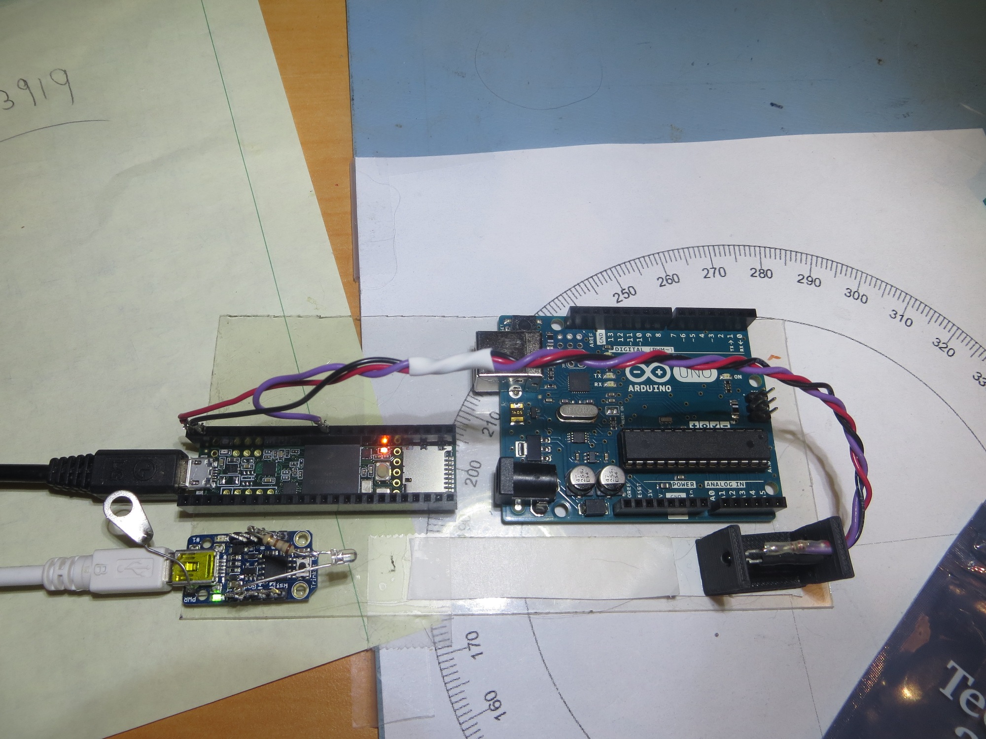
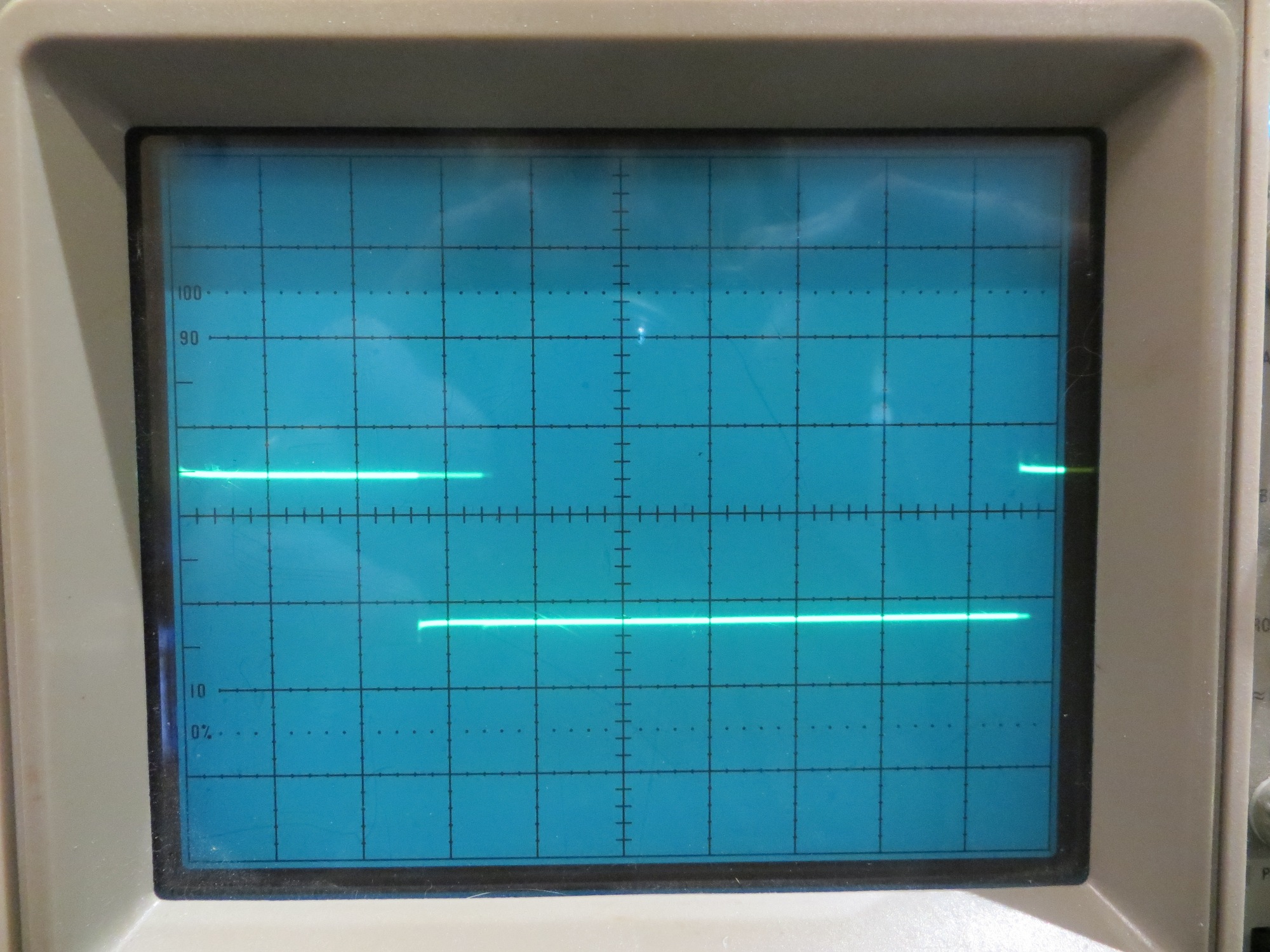
My friend and mentor John Jenkins, who has been looking over my shoulder (and occasionally whacking me on the head) during this project, was unsure that my frequency matching setup was actually 100% complete, as the video I took the last time didn’t run long enough to convince him (and there were some un-explained triggering glitches as well). So, I thought I would re-do this part to make him happy. To do this I modified my little test program from the above ‘rabbit-hole’ elapsedMicros issue to output a square wave from the demodulator board that could be compared to the transmitter square wave.
As shown in the above video, the transmit and demodulator frequencies are quite well matched, showing essentially zero relative drift even over the 30-40 second time of the video. Mission accomplished! ;-).
Sample Acquisition Step:
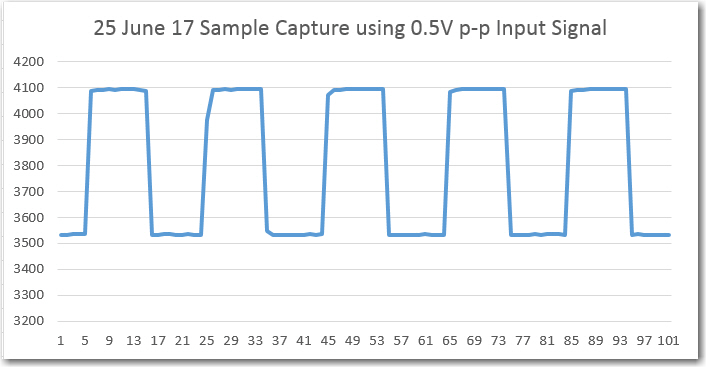
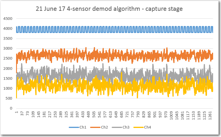
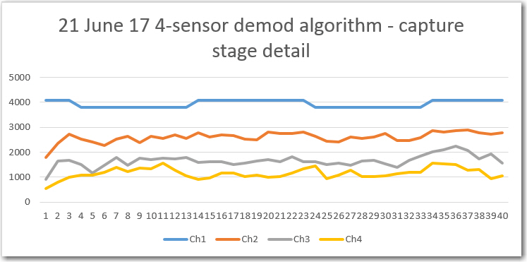
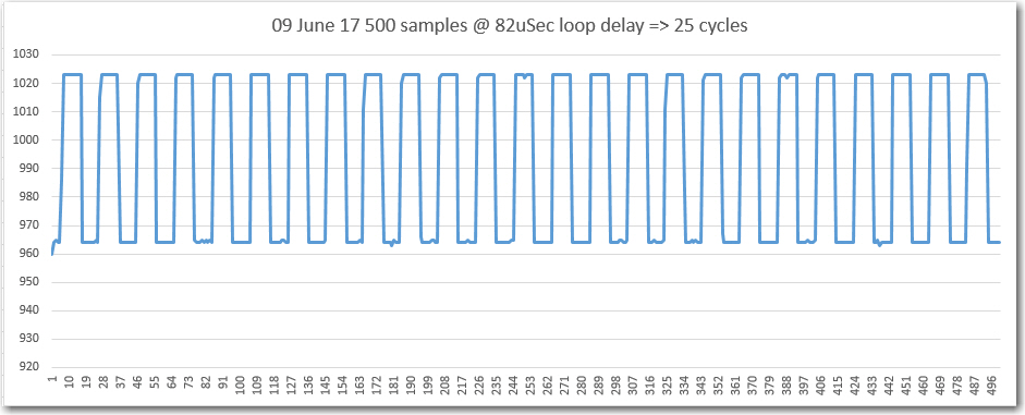
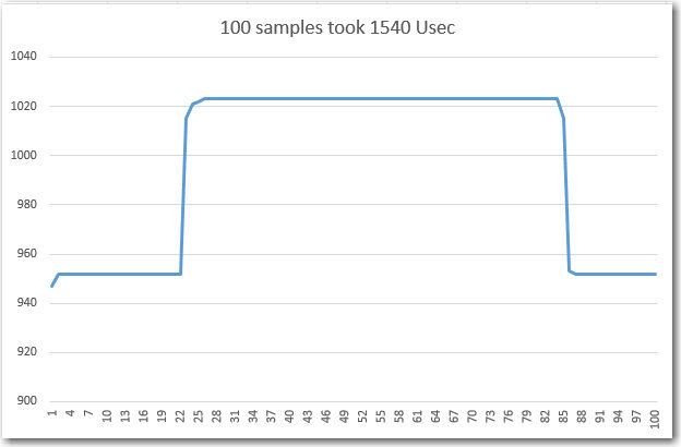
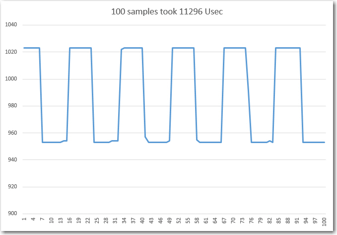
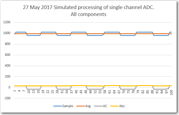
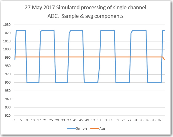
I modified my demodulator program to properly initialize the ‘elapsedMicros’ variable being used for sample timing, and verified proper operation by commenting out everything but the sample acquisition step. I captured several hundred samples, and plotted the first hundred in Excel as follows:
100 samples using proper ‘elapsedMicros’ variable initialization
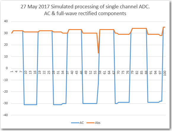
Sample Sum Step:
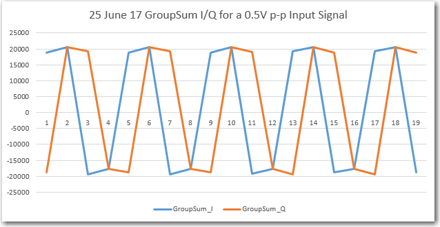
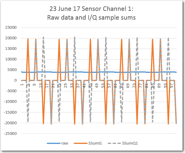
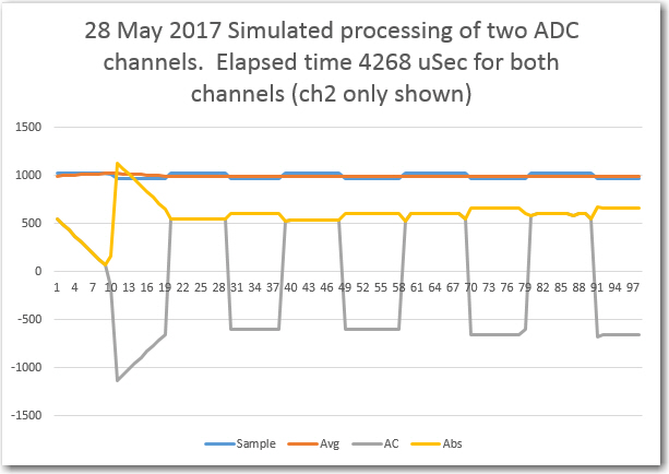
Next, each group of five samples (1/4 cycle) is summed, and the ‘In-phase’ and ‘Quadrature’ components are generated using the appropriate sign sequences. As shown in the following, this appears to be happening correctly:
|
1 2 3 4 5 6 7 8 9 10 11 12 13 14 15 16 17 18 19 20 21 22 23 24 25 26 27 28 29 30 31 32 33 34 35 36 37 38 39 40 41 42 43 44 45 46 47 48 49 50 51 52 53 54 55 56 57 58 59 60 61 62 63 64 65 66 67 68 69 70 71 72 73 74 75 76 77 78 79 80 81 82 83 84 85 86 87 88 89 90 91 92 93 94 95 96 97 98 99 100 101 102 103 104 105 106 107 108 109 110 111 112 113 114 115 116 117 118 119 120 121 122 123 124 125 126 127 128 129 130 131 132 133 134 135 136 137 138 139 140 141 142 143 144 145 146 147 148 149 150 151 152 153 154 155 156 157 158 159 160 161 162 163 164 165 166 167 168 169 170 171 172 173 174 175 176 177 178 179 180 181 182 183 184 185 186 187 188 189 190 191 192 193 194 195 196 197 198 199 200 201 202 203 204 205 206 207 208 209 210 211 212 213 214 215 216 217 218 219 220 221 222 223 224 225 226 227 228 229 230 231 232 233 234 235 236 237 238 239 240 241 242 243 244 245 246 247 248 249 250 251 252 253 254 255 256 257 258 259 260 261 262 263 264 265 266 267 268 269 270 271 272 273 274 275 276 277 278 279 280 281 282 283 284 285 286 287 288 289 290 291 292 293 294 295 296 297 298 299 300 301 302 303 304 305 306 307 308 309 310 311 312 313 314 315 316 317 318 319 320 321 322 323 324 325 326 327 328 329 330 331 332 333 334 335 336 337 338 339 340 341 342 343 344 345 346 347 348 349 350 351 352 353 354 355 356 357 358 359 360 361 362 363 364 365 366 367 368 369 370 371 372 373 374 375 376 377 378 379 380 |
Opening port Port open SI Samp GSumI GSumQ 0 4089 1 4091 2 4092 3 4095 4 3392 19759 -19759 5 3390 6 3395 7 3390 8 3389 9 3390 16954 16954 10 3388 11 3388 12 3390 13 3387 14 4081 -17634 17634 15 4090 16 4093 17 4092 18 4093 19 4093 -20461 -20461 20 4089 21 4092 22 4095 23 4095 24 3400 19771 -19771 25 3387 26 3391 27 3386 28 3389 29 3389 16942 16942 30 3388 31 3389 32 3386 33 3383 34 3756 -17302 17302 35 4090 36 4090 37 4092 38 4091 39 4091 -20454 -20454 40 4095 41 4095 42 4094 43 4093 44 4093 20470 -20470 45 3389 46 3389 47 3386 48 3391 49 3391 16946 16946 50 3391 51 3389 52 3392 53 3390 54 3388 -16950 16950 55 4089 56 4092 57 4095 58 4093 59 4094 -20463 -20463 60 4093 61 4095 62 4093 63 4095 64 4095 20471 -20471 65 3391 66 3392 67 3386 68 3390 69 3395 16954 16954 70 3388 71 3387 72 3387 73 3395 74 3391 -16948 16948 75 4085 76 4095 77 4092 78 4095 79 4093 -20460 -20460 80 4091 81 4095 82 4088 83 4090 84 4095 20459 -20459 85 3391 86 3386 87 3390 88 3387 89 3386 16940 16940 90 3389 91 3390 92 3389 93 3387 94 3387 -16942 16942 95 4047 96 4081 97 4082 98 4090 99 4095 -20395 -20395 100 4095 101 4095 102 4095 103 4095 104 4095 20475 -20475 105 4094 106 3390 107 3391 108 3390 109 3387 17652 17652 110 3386 111 3387 112 3386 113 3389 114 3391 -16939 16939 115 3394 116 4088 117 4090 118 4090 119 4093 -19755 -19755 120 4093 121 4090 122 4094 123 4095 124 4091 20463 -20463 125 4095 126 3388 127 3390 128 3389 129 3390 17652 17652 130 3391 131 3387 132 3387 133 3386 134 3390 -16941 16941 135 3390 136 4094 137 4094 138 4091 139 4094 -19763 -19763 140 4093 141 4095 142 4093 143 4093 144 4095 20469 -20469 145 4094 146 3385 147 3389 148 3391 149 3387 17646 17646 150 3387 151 3389 152 3390 153 3390 154 3386 -16942 16942 155 3382 156 4072 157 4089 158 4093 159 4092 -19728 -19728 160 4095 161 4094 162 4095 163 4095 164 4093 20472 -20472 165 4095 166 3450 167 3395 168 3394 169 3390 17724 17724 170 3392 171 3389 172 3390 173 3384 174 3389 -16944 16944 175 3389 176 3389 177 4093 178 4093 179 4090 -19054 -19054 180 4095 181 4095 182 4095 183 4094 184 4095 20474 -20474 185 4091 186 4095 187 3390 188 3387 189 3389 18352 18352 190 3390 191 3390 192 3389 193 3389 194 3388 -16946 16946 195 3388 196 3387 197 4091 198 4088 199 4091 -19045 -19045 200 4093 201 4094 202 4095 203 4095 204 4095 20472 -20472 205 4093 206 4093 207 3393 208 3386 209 3389 18354 18354 210 3388 211 3386 212 3389 213 3391 214 3389 -16943 16943 215 3388 216 3391 217 4080 218 4091 219 4095 -19045 -19045 220 4095 221 4095 222 4091 223 4095 224 4095 20471 -20471 225 4094 226 4089 227 3395 228 3390 229 3385 18353 18353 230 3386 231 3396 232 3387 233 3389 234 3391 -16949 16949 235 3387 236 3388 237 3858 238 4094 239 4091 -18818 -18818 240 4091 241 4095 242 4095 243 4095 244 4095 20471 -20471 245 4094 246 4089 247 4094 248 3401 249 3386 19064 19064 250 3388 251 3389 252 3393 253 3386 254 3390 -16946 16946 255 3390 256 3390 257 3392 258 4087 259 4090 -18349 -18349 260 4092 261 4094 262 4093 263 4095 264 4091 20465 -20465 265 4090 266 4095 267 4090 268 3394 269 3389 19058 19058 270 3391 271 3388 272 3390 273 3387 274 3385 -16941 16941 275 3386 276 3387 277 3389 278 4084 279 4095 -18341 -18341 280 4091 281 4093 282 4094 283 4093 284 4095 20466 -20466 285 4088 286 4093 287 4091 288 3388 289 3388 19048 19048 290 3390 291 3389 292 3389 293 3391 294 3388 -16947 16947 295 3389 296 3387 297 3387 298 4048 299 4089 -18300 -18300 300 4090 301 4092 302 4095 303 4094 304 4092 20463 -20463 305 4094 306 4092 307 4093 308 3761 309 3391 19431 19431 310 3387 311 3390 312 3390 313 3390 314 3388 -16945 16945 315 3388 316 3387 317 3384 318 3390 319 4088 -17637 -17637 320 4093 321 4095 322 4094 323 4095 324 4095 20472 -20472 325 4095 326 4095 327 4095 328 4095 329 3390 19770 19770 330 3391 331 3386 332 3387 333 3387 334 3390 -16941 16941 335 3389 336 3387 337 3392 338 3389 339 4086 -17643 -17643 340 4091 341 4095 342 4094 343 4095 344 4093 20468 -20468 345 4093 346 4092 347 4090 348 4095 349 3391 19761 19761 350 3388 351 3390 352 3395 353 3391 354 3387 -16951 16951 355 3386 356 3388 357 3388 358 3388 359 4072 -17622 -17622 360 4092 361 4091 362 4092 363 4095 364 4092 20462 -20462 365 4091 366 4095 367 4095 368 4092 369 3408 19781 19781 370 3389 371 3389 372 3389 373 3389 374 3389 -16945 16945 Port closed |
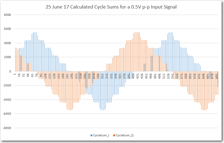
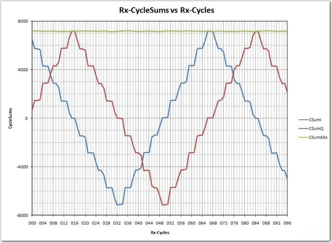
Cycle Sum Accumulation:
As each sample group is summed and the I/Q components generated, accumulate the 1/4-cycle I/Q sums into a ‘Cycle Sum’. As the following printout shows, this step also is being performed properly
|
1 2 3 4 5 6 7 8 9 10 11 12 13 14 15 16 17 18 19 20 21 22 23 24 25 26 27 28 29 30 31 32 33 34 35 36 37 38 39 40 41 42 43 44 45 46 47 48 49 50 51 52 53 54 55 56 57 58 59 60 61 62 63 64 65 66 67 68 69 70 71 72 73 74 75 76 77 78 79 80 81 82 83 84 85 86 87 88 89 90 91 92 93 94 95 96 97 98 99 100 101 102 103 104 105 106 107 108 109 110 111 112 113 114 115 116 117 118 119 |
Opening port Port open SI Samp GSumI GSumQ CSumI CSumQ 1 3382 2 3384 3 3386 4 3384 5 3382 16918 -16918 16918 -16918 6 3384 7 4027 8 4089 9 4095 10 4091 19686 19686 36604 2768 11 4095 12 4095 13 4095 14 4093 15 4093 -20471 20471 16133 23239 16 4093 17 3699 18 3387 19 3376 20 3388 -17943 -17943 -1810 5296 21 3383 22 3385 23 3385 24 3385 25 3384 16922 -16922 16922 -16922 26 3384 27 3384 28 4092 29 4095 30 4095 19050 19050 35972 2128 31 4089 32 4095 33 4095 34 4095 35 4094 -20468 20468 15504 22596 36 4092 37 4092 38 3387 39 3384 40 3390 -18345 -18345 -2841 4251 41 3383 42 3384 43 3383 44 3384 45 3383 16917 -16917 16917 -16917 46 3383 47 3386 48 4085 49 4093 50 4093 19040 19040 35957 2123 51 4095 52 4095 53 4094 54 4095 55 4095 -20474 20474 15483 22597 56 4093 57 4095 58 3383 59 3386 60 3387 -18344 -18344 -2861 4253 61 3384 62 3385 63 3382 64 3384 65 3384 16919 -16919 16919 -16919 66 3387 67 3385 68 4087 69 4090 70 4093 19042 19042 35961 2123 71 4095 72 4095 73 4093 74 4094 75 4091 -20468 20468 15493 22591 76 4094 77 4089 78 3408 79 3385 80 3386 -18362 -18362 -2869 4229 81 3385 82 3383 83 3385 84 3383 85 3386 16922 -16922 16922 -16922 86 3385 87 3384 88 3637 89 4086 90 4090 18582 18582 35504 1660 91 4091 92 4093 93 4095 94 4092 95 4095 -20466 20466 15038 22126 96 4093 97 4095 98 4095 99 3387 100 3383 -19053 -19053 -4015 3073 101 3385 102 3388 103 3387 104 3387 105 3383 16930 -16930 16930 -16930 106 3381 107 3386 108 3386 109 4087 110 4091 18331 18331 35261 1401 111 4094 112 4093 113 4083 114 4091 Port closed |
Running Sum Accumulation:
The last step in the algorithm is to compute the N-cycle running sum of all the cycle sums. This is done by subtracting the oldest value from the circular buffer from the current running sum, adding the current cycle sum to the running sum, and then replacing the oldest cycle sum value in the circular buffer by the current cycle sum.
- RunningSum = RunningSum + CurrentCycleSum – OldestCycleSum
- OldestCycleSum = CurrentCycleSum
- Circular buffer index incremented by 1 (MOD N)
This one took a while to instrument properly. I first tried just adding some more columns on to the current display setup, but that became too cumbersome, too fast. Verifying the running sum calculation requires looking at not only the current running sum, but also its value from N cycles (or N*5*4 samples) previously. So, I modified the code to only print one line per cycle, and this was much easier to manage. Here’s a partial printout showing a little over 200 cycles, representing about 400mSec (200 cycles * 2mSec/cycle).
|
1 2 3 4 5 6 7 8 9 10 11 12 13 14 15 16 17 18 19 20 21 22 23 24 25 26 27 28 29 30 31 32 33 34 35 36 37 38 39 40 41 42 43 44 45 46 47 48 49 50 51 52 53 54 55 56 57 58 59 60 61 62 63 64 65 66 67 68 69 70 71 72 73 74 75 76 77 78 79 80 81 82 83 84 85 86 87 88 89 90 91 92 93 94 95 96 97 98 99 100 101 102 103 104 105 106 107 108 109 110 111 112 113 114 115 116 117 118 119 120 121 122 123 124 125 126 127 128 129 130 131 132 133 134 135 136 137 138 139 140 141 142 143 144 145 146 147 148 149 150 151 152 153 154 155 156 157 158 159 160 161 162 163 164 165 166 167 168 169 170 171 172 173 174 175 176 177 178 179 180 181 182 183 184 185 186 187 188 189 190 191 192 193 194 195 196 197 198 199 200 201 202 203 204 205 206 207 208 209 210 211 212 213 214 215 216 217 218 219 220 221 222 223 224 225 226 227 228 229 230 231 232 |
RSI CSumI CSumQ OldRSI OldRSQ CurRSI CurRQ NewRSI NewRSQ FinVal 0 6523 657 0 0 0 0 6523 657 7180 1 5737 1453 0 0 6523 657 12260 2110 14370 2 5718 1444 0 0 12260 2110 17978 3554 21532 3 5647 1515 0 0 17978 3554 23625 5069 28694 4 4290 2860 0 0 23625 5069 27915 7929 35844 5 4281 2887 0 0 27915 7929 32196 10816 43012 6 4250 2906 0 0 32196 10816 36446 13722 50168 7 3472 3698 0 0 36446 13722 39918 17420 57338 8 2869 4311 0 0 39918 17420 42787 21731 64518 9 2838 4306 0 0 42787 21731 45625 26037 71662 10 2527 4617 0 0 45625 26037 48152 30654 78806 11 1410 5728 0 0 48152 30654 49562 36382 85944 12 1416 5750 0 0 49562 36382 50978 42132 93110 13 1389 5751 0 0 50978 42132 52367 47883 100250 14 450 6664 0 0 52367 47883 52817 54547 107364 15 -21 7155 0 0 52817 54547 52796 61702 114498 16 -14 7166 0 0 52796 61702 52782 68868 121650 17 -771 6403 0 0 52782 68868 52011 75271 127282 18 -1466 5718 0 0 52011 75271 50545 80989 131534 19 -1461 5717 0 0 50545 80989 49084 86706 135790 20 -1597 5577 0 0 49084 86706 47487 92283 139770 21 -2853 4315 0 0 47487 92283 44634 96598 141232 22 -2876 4292 0 0 44634 96598 41758 100890 142648 23 -2903 4283 0 0 41758 100890 38855 105173 144028 24 -3678 3476 0 0 38855 105173 35177 108649 143826 25 -4302 2838 0 0 35177 108649 30875 111487 142362 26 -4320 2842 0 0 30875 111487 26555 114329 140884 27 -4738 2424 0 0 26555 114329 21817 116753 138570 28 -5754 1424 0 0 21817 116753 16063 118177 134240 29 -5745 1415 0 0 16063 118177 10318 119592 129910 30 -5745 1373 0 0 10318 119592 4573 120965 125538 31 -6611 545 0 0 4573 120965 -2038 121510 123548 32 -7148 0 0 0 -2038 121510 -9186 121510 130696 33 -7143 -19 0 0 -9186 121510 -16329 121491 137820 34 -7100 -76 0 0 -16329 121491 -23429 121415 144844 35 -5724 -1456 0 0 -23429 121415 -29153 119959 149112 36 -5738 -1464 0 0 -29153 119959 -34891 118495 153386 37 -5714 -1468 0 0 -34891 118495 -40605 117027 157632 38 -4882 -2302 0 0 -40605 117027 -45487 114725 160212 39 -4284 -2876 0 0 -45487 114725 -49771 111849 161620 40 -4285 -2871 0 0 -49771 111849 -54056 108978 163034 41 -4096 -3064 0 0 -54056 108978 -58152 105914 164066 42 -2848 -4322 0 0 -58152 105914 -61000 101592 162592 43 -2846 -4316 0 0 -61000 101592 -63846 97276 161122 44 -2822 -4328 0 0 -63846 97276 -66668 92948 159616 45 -1575 -5587 0 0 -66668 92948 -68243 87361 155604 46 -1420 -5740 0 0 -68243 87361 -69663 81621 151284 47 -1402 -5736 0 0 -69663 81621 -71065 75885 146950 48 -673 -6455 0 0 -71065 75885 -71738 69430 141168 49 11 -7161 0 0 -71738 69430 -71727 62269 133996 50 20 -7158 0 0 -71727 62269 -71707 55111 126818 51 77 -7109 0 0 -71707 55111 -71630 48002 119632 52 1446 -5724 0 0 -71630 48002 -70184 42278 112462 53 1456 -5718 0 0 -70184 42278 -68728 36560 105288 54 1464 -5708 0 0 -68728 36560 -67264 30852 98116 55 2291 -4881 0 0 -67264 30852 -64973 25971 90944 56 2874 -4276 0 0 -64973 25971 -62099 21695 83794 57 2887 -4279 0 0 -62099 21695 -59212 17416 76628 58 3001 -4177 0 0 -59212 17416 -56211 13239 69450 59 4314 -2848 0 0 -56211 13239 -51897 10391 62288 60 4319 -2855 0 0 -51897 10391 -47578 7536 55114 61 4359 -2819 0 0 -47578 7536 -43219 4717 47936 62 5670 -1480 0 0 -43219 4717 -37549 3237 40786 63 5749 -1415 0 0 -37549 3237 -31800 1822 33622 0 5741 -1413 6523 657 -31800 1822 -32582 -248 32830 -32582 -248 1 6401 -737 5737 1453 -32582 -248 -31918 -2438 34356 -31918 -2438 2 7167 17 5718 1444 -31918 -2438 -30469 -3865 34334 3 7155 21 5647 1515 -30469 -3865 -28961 -5359 34320 4 7146 12 4290 2860 -28961 -5359 -26105 -8207 34312 5 6377 781 4281 2887 -26105 -8207 -24009 -10313 34322 6 5729 1439 4250 2906 -24009 -10313 -22530 -11780 34310 7 5722 1460 3472 3698 -22530 -11780 -20280 -14018 34298 8 5393 1763 2869 4311 -20280 -14018 -17756 -16566 34322 9 4288 2872 2838 4306 -17756 -16566 -16306 -18000 34306 10 4289 2865 2527 4617 -16306 -18000 -14544 -19752 34296 11 4264 2898 1410 5728 -14544 -19752 -11690 -22582 34272 12 3152 4006 1416 5750 -11690 -22582 -9954 -24326 34280 13 2843 4315 1389 5751 -9954 -24326 -8500 -25762 34262 14 2842 4318 450 6664 -8500 -25762 -6108 -28108 34216 15 2092 5086 -21 7155 -6108 -28108 -3995 -30177 34172 16 1410 5754 -14 7166 -3995 -30177 -2571 -31589 34160 17 1414 5742 -771 6403 -2571 -31589 -386 -32250 32636 18 1340 5828 -1466 5718 -386 -32250 2420 -32140 34560 19 302 6824 -1461 5717 2420 -32140 4183 -31033 35216 20 5 7127 -1597 5577 4183 -31033 5785 -29483 35268 21 -30 7152 -2853 4315 5785 -29483 8608 -26646 35254 22 -832 6346 -2876 4292 8608 -26646 10652 -24592 35244 23 -1462 5718 -2903 4283 10652 -24592 12093 -23157 35250 24 -1455 5725 -3678 3476 12093 -23157 14316 -20908 35224 25 -1678 5532 -4302 2838 14316 -20908 16940 -18214 35154 26 -2884 4300 -4320 2842 16940 -18214 18376 -16756 35132 27 -2888 4280 -4738 2424 18376 -16756 20226 -14900 35126 28 -2874 4270 -5754 1424 20226 -14900 23106 -12054 35160 29 -3818 3342 -5745 1415 23106 -12054 25033 -10127 35160 30 -4309 2859 -5745 1373 25033 -10127 26469 -8641 35110 31 -4330 2842 -6611 545 26469 -8641 28750 -6344 35094 32 -4987 2167 -7148 0 28750 -6344 30911 -4177 35088 33 -5751 1419 -7143 -19 30911 -4177 32303 -2739 35042 34 -5749 1415 -7100 -76 32303 -2739 33654 -1248 34902 35 -5836 1310 -5724 -1456 33654 -1248 33542 1518 35060 36 -7155 -5 -5738 -1464 33542 1518 32125 2977 35102 37 -7144 2 -5714 -1468 32125 2977 30695 4447 35142 38 -7143 -23 -4882 -2302 30695 4447 28434 6726 35160 39 -7058 -108 -4284 -2876 28434 6726 25660 9494 35154 40 -5731 -1449 -4285 -2871 25660 9494 24214 10916 35130 41 -5720 -1448 -4096 -3064 24214 10916 22590 12532 35122 42 -5688 -1478 -2848 -4322 22590 12532 19750 15376 35126 43 -4482 -2690 -2846 -4316 19750 15376 18114 17002 35116 44 -4301 -2891 -2822 -4328 18114 17002 16635 18439 35074 45 -4271 -2891 -1575 -5587 16635 18439 13939 21135 35074 46 -3900 -3270 -1420 -5740 13939 21135 11459 23605 35064 47 -2858 -4322 -1402 -5736 11459 23605 10003 25019 35022 48 -2834 -4300 -673 -6455 10003 25019 7842 27174 35016 49 -2812 -4342 11 -7161 7842 27174 5019 29993 35012 50 -1457 -5689 20 -7158 5019 29993 3542 31462 35004 51 -1402 -5746 77 -7109 3542 31462 2063 32825 34888 52 -1400 -5760 1446 -5724 2063 32825 -783 32789 33572 53 -670 -6466 1456 -5718 -783 32789 -2909 32041 34950 54 20 -7162 1464 -5708 -2909 32041 -4353 30587 34940 55 34 -7142 2291 -4881 -4353 30587 -6610 28326 34936 56 92 -7092 2874 -4276 -6610 28326 -9392 25510 34902 57 1441 -5717 2887 -4279 -9392 25510 -10838 24072 34910 58 1455 -5713 3001 -4177 -10838 24072 -12384 22536 34920 59 1475 -5703 4314 -2848 -12384 22536 -15223 19681 34904 60 2494 -4690 4319 -2855 -15223 19681 -17048 17846 34894 61 2889 -4287 4359 -2819 -17048 17846 -18518 16378 34896 62 2883 -4281 5670 -1480 -18518 16378 -21305 13577 34882 63 3491 -3681 5749 -1415 -21305 13577 -23563 11311 34874 0 4306 -2846 5741 -1413 -23563 11311 -24998 9878 34876 1 4320 -2838 6401 -737 -24998 9878 -27079 7777 34856 2 4339 -2809 7167 17 -27079 7777 -29907 4951 34858 3 5733 -1437 7155 21 -29907 4951 -31329 3493 34822 4 5738 -1414 7146 12 -31329 3493 -32737 2067 34804 5 5762 -1398 6377 781 -32737 2067 -33352 -112 33464 6 6609 -561 5729 1439 -33352 -112 -32472 -2112 34584 7 7145 1 5722 1460 -32472 -2112 -31049 -3571 34620 8 7149 -1 5393 1763 -31049 -3571 -29293 -5335 34628 9 7128 42 4288 2872 -29293 -5335 -26453 -8165 34618 10 6252 918 4289 2865 -26453 -8165 -24490 -10112 34602 11 5736 1452 4264 2898 -24490 -10112 -23018 -11558 34576 12 5707 1453 3152 4006 -23018 -11558 -20463 -14111 34574 13 5099 2079 2843 4315 -20463 -14111 -18207 -16347 34554 14 4306 2882 2842 4318 -18207 -16347 -16743 -17783 34526 15 4280 2862 2092 5086 -16743 -17783 -14555 -20007 34562 16 4212 2932 1410 5754 -14555 -20007 -11753 -22829 34582 17 2889 4261 1414 5742 -11753 -22829 -10278 -24310 34588 18 2857 4323 1340 5828 -10278 -24310 -8761 -25815 34576 19 2834 4318 302 6824 -8761 -25815 -6229 -28321 34550 20 2074 5088 5 7127 -6229 -28321 -4160 -30360 34520 21 1421 5735 -30 7152 -4160 -30360 -2709 -31777 34486 22 1416 5728 -832 6346 -2709 -31777 -461 -32395 32856 23 1235 5895 -1462 5718 -461 -32395 2236 -32218 34454 24 -19 7151 -1455 5725 2236 -32218 3672 -30792 34464 25 -19 7153 -1678 5532 3672 -30792 5331 -29171 34502 26 -29 7139 -2884 4300 5331 -29171 8186 -26332 34518 27 -893 6297 -2888 4280 8186 -26332 10181 -24315 34496 28 -1467 5723 -2874 4270 10181 -24315 11588 -22862 34450 29 -1459 5723 -3818 3342 11588 -22862 13947 -20481 34428 30 -1962 5192 -4309 2859 13947 -20481 16294 -18148 34442 31 -2877 4273 -4330 2842 16294 -18148 17747 -16717 34464 32 -2885 4269 -4987 2167 17747 -16717 19849 -14615 34464 33 -2943 4219 -5751 1419 19849 -14615 22657 -11815 34472 34 -4228 2954 -5749 1415 22657 -11815 24178 -10276 34454 35 -4321 2859 -5836 1310 24178 -10276 25693 -8727 34420 36 -4346 2860 -7155 -5 25693 -8727 28502 -5862 34364 37 -5080 2096 -7144 2 28502 -5862 30566 -3768 34334 38 -5735 1413 -7143 -23 30566 -3768 31974 -2332 34306 39 -5747 1423 -7058 -108 31974 -2332 33285 -801 34086 40 -6155 1007 -5731 -1449 33285 -801 32861 1655 34516 41 -7177 -17 -5720 -1448 32861 1655 31404 3086 34490 42 -7144 -12 -5688 -1478 31404 3086 29948 4552 34500 43 -7155 -3 -4482 -2690 29948 4552 27275 7239 34514 44 -6818 -348 -4301 -2891 27275 7239 24758 9782 34540 45 -5729 -1445 -4271 -2891 24758 9782 23300 11228 34528 46 -5714 -1454 -3900 -3270 23300 11228 21486 13044 34530 47 -5667 -1503 -2858 -4322 21486 13044 18677 15863 34540 48 -4279 -2881 -2834 -4300 18677 15863 17232 17282 34514 49 -4289 -2887 -2812 -4342 17232 17282 15755 18737 34492 50 -4279 -2891 -1457 -5689 15755 18737 12933 21535 34468 51 -3507 -3639 -1402 -5746 12933 21535 10828 23642 34470 52 -2843 -4305 -1400 -5760 10828 23642 9385 25097 34482 53 -2832 -4334 -670 -6466 9385 25097 7223 27229 34452 54 -2774 -4384 20 -7162 7223 27229 4429 30007 34436 55 -1420 -5726 34 -7142 4429 30007 2975 31423 34398 56 -1424 -5736 92 -7092 2975 31423 1459 32779 34238 57 -1403 -5759 1441 -5717 1459 32779 -1385 32737 34122 58 -554 -6596 1455 -5713 -1385 32737 -3394 31854 35248 59 18 -7160 1475 -5703 -3394 31854 -4851 30397 35248 60 18 -7154 2494 -4690 -4851 30397 -7327 27933 35260 61 234 -6950 2889 -4287 -7327 27933 -9982 25270 35252 62 1449 -5737 2883 -4281 -9982 25270 -11416 23814 35230 63 1444 -5692 3491 -3681 -11416 23814 -13463 21803 35266 0 1484 -5686 4306 -2846 -13463 21803 -16285 18963 35248 1 2874 -4296 4320 -2838 -16285 18963 -17731 17505 35236 2 2896 -4286 4339 -2809 -17731 17505 -19174 16028 35202 3 2888 -4282 5733 -1437 -19174 16028 -22019 13183 35202 4 3695 -3481 5738 -1414 -22019 13183 -24062 11116 35178 5 4298 -2850 5762 -1398 -24062 11116 -25526 9664 35190 6 4310 -2846 6609 -561 -25526 9664 -27825 7379 35204 7 4415 -2729 7145 1 -27825 7379 -30555 4649 35204 8 5742 -1408 7149 -1 -30555 4649 -31962 3242 35204 9 5749 -1421 7128 42 -31962 3242 -33341 1779 35120 10 5772 -1404 6252 918 -33341 1779 -33821 -543 34364 11 6994 -176 5736 1452 -33821 -543 -32563 -2171 34734 12 7146 8 5707 1453 -32563 -2171 -31124 -3616 34740 13 7154 10 5099 2079 -31124 -3616 -29069 -5685 34754 14 7132 52 4306 2882 -29069 -5685 -26243 -8515 34758 15 5983 1191 4280 2862 -26243 -8515 -24540 -10186 34726 16 5730 1440 4212 2932 -24540 -10186 -23022 -11678 34700 17 5717 1451 2889 4261 -23022 -11678 -20194 -14488 34682 18 4965 2211 2857 4323 -20194 -14488 -18086 -16600 34686 19 4300 2890 2834 4318 -18086 -16600 -16620 -18028 34648 20 4278 2880 2074 5088 -16620 -18028 -14416 -20236 34652 21 4142 3016 1421 5735 -14416 -20236 -11695 -22955 34650 22 2858 4308 1416 5728 -11695 -22955 -10253 -24375 34628 23 2853 4289 1235 5895 -10253 -24375 -8635 -25981 34616 24 2820 4336 -19 7151 -8635 -25981 -5796 -28796 34592 25 2049 5121 -19 7153 -5796 -28796 -3728 -30828 34556 26 1410 5738 -29 7139 -3728 -30828 -2289 -32229 34518 27 1420 5732 -893 6297 -2289 -32229 24 -32794 32818 28 1020 6138 -1467 5723 24 -32794 2511 -32379 34890 29 -23 7173 -1459 5723 2511 -32379 3947 -30929 34876 30 -28 7138 -1962 5192 3947 -30929 5881 -28983 34864 31 -38 7124 -2877 4273 5881 -28983 8720 -26132 34852 32 -1075 6107 -2885 4269 8720 -26132 10530 -24294 34824 33 -1443 5721 -2943 4219 10530 -24294 12030 -22792 34822 34 -1457 5715 -4228 2954 12030 -22792 14801 -20031 34832 35 -2203 4975 -4321 2859 14801 -20031 16919 -17915 34834 36 -2889 4279 -4346 2860 16919 -17915 18376 -16496 34872 37 -2881 4281 -5080 2096 18376 -16496 20575 -14311 34886 38 -2956 4176 -5735 1413 20575 -14311 23354 -11548 34902 |
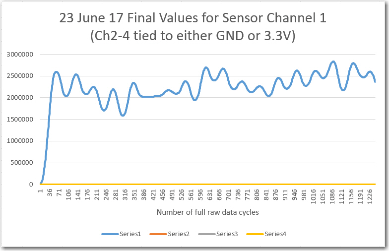
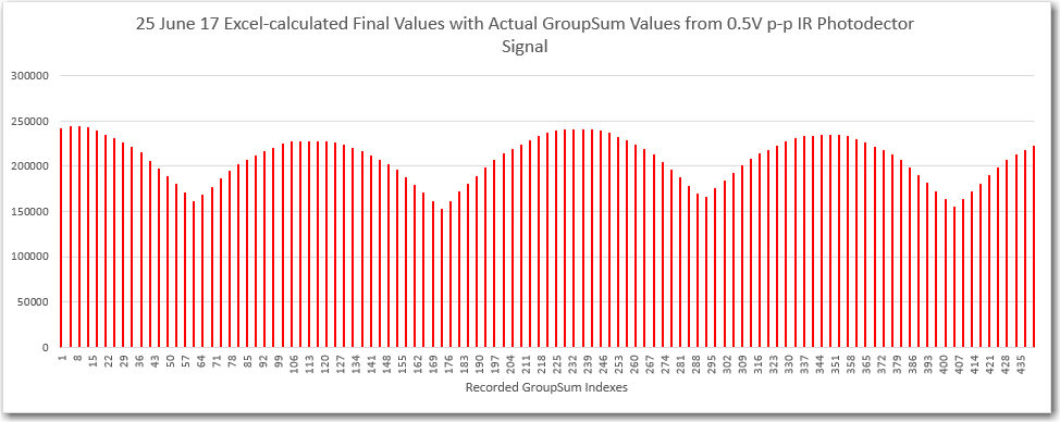
To analyze these results, I dropped them into Excel, and used it’s ‘Freeze Panes’ feature to juxtapose the results from cycles 0 through 4 with cycles 65, 66, and 67. This allowed me to verify that the running sum expression was being calculated correctly and the circular buffer was being loaded and referenced correctly. When I finished verifying these results, I plotted the final value column, as shown below:
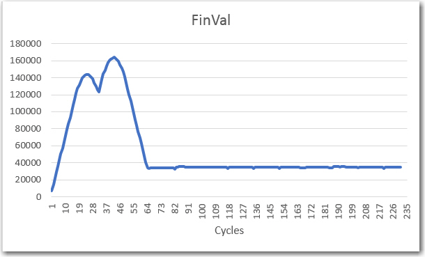
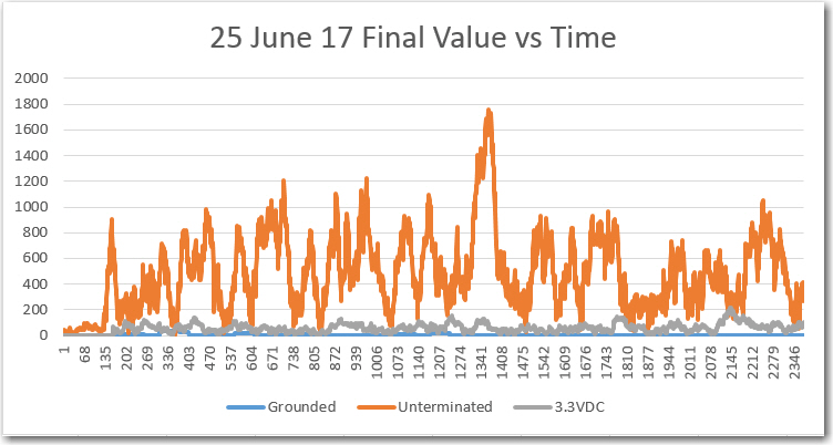
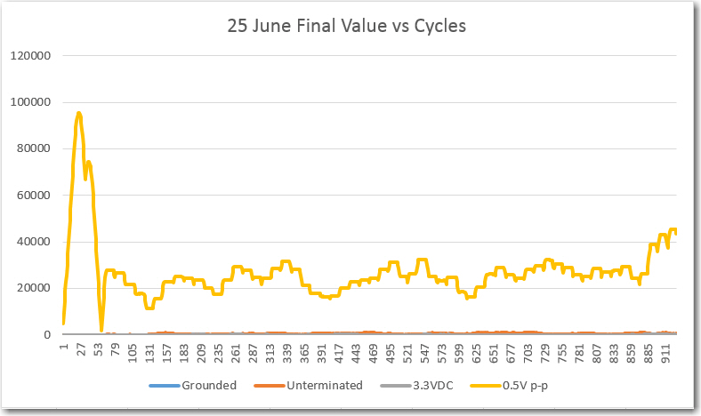
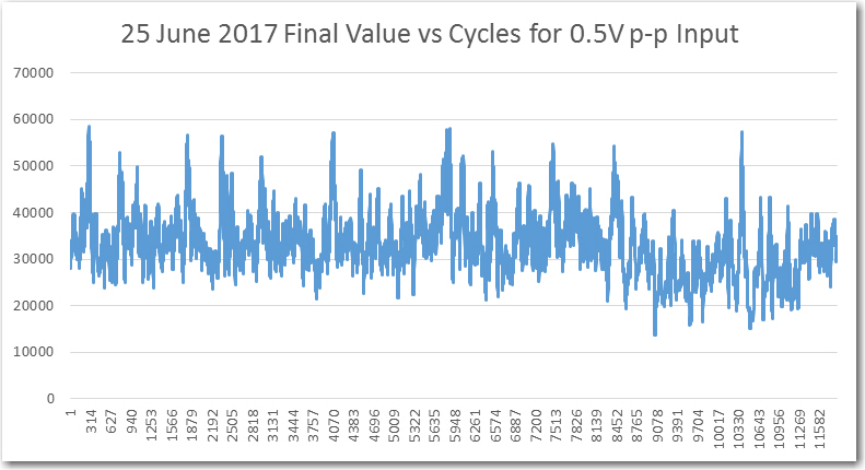
New ‘Final Value’ results
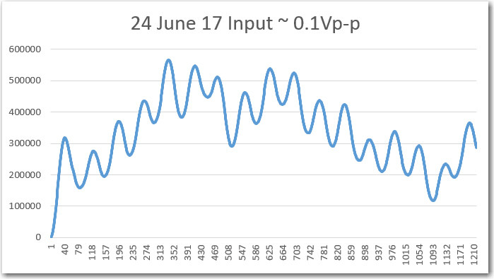
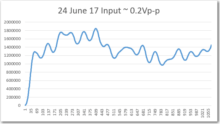
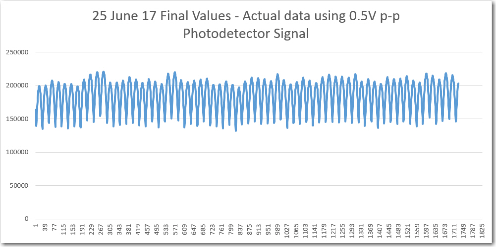
As an experiment, I also momentarily blocked the IR path with my finger, and plotted the results, as shown below:
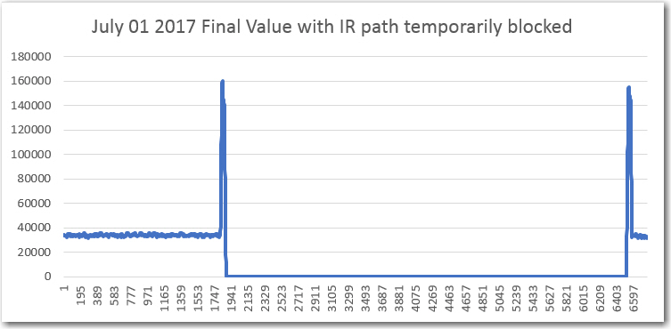
Filter response with finger blocking IR path for a few seconds, then removed
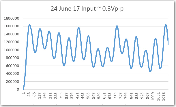
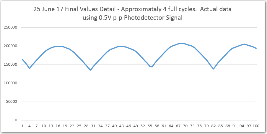
And again, just waving my finger into and out of the IR path several times over several seconds
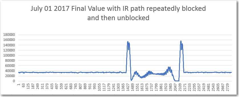
Filter response with finger moved in and out of IR path several times over 3-5 seconds
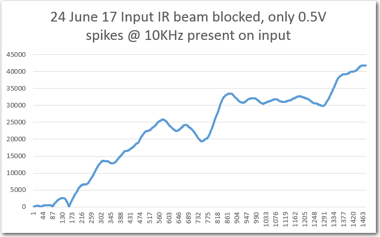
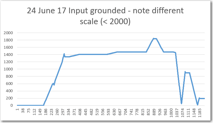
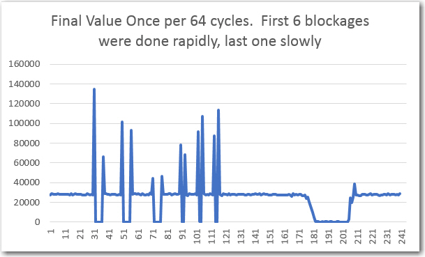
John’s comment on all this was “still not right”, as explained below:
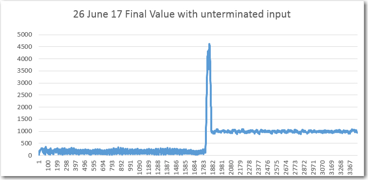
My take on the above was that it is the print statements that are the cause of the problem, not anything to do with Teensy ADC speed. To test this theory, I removed all but the ‘Final Value’ print statement, and put that one statement in a block that executed only once per 64 cycles. With this change, I could see that the print output was keeping up with real time and not lagging as before. Below shows a plot with several IR beam block/unblock cycles, and it appears that the ‘Final Value’ output is much more responsive to the block/unblock events. Interestingly, it appears there is some sort of Gibbs phenomenon associated with the ‘fast’ cycles when the system switches between one equilibrium level and another.
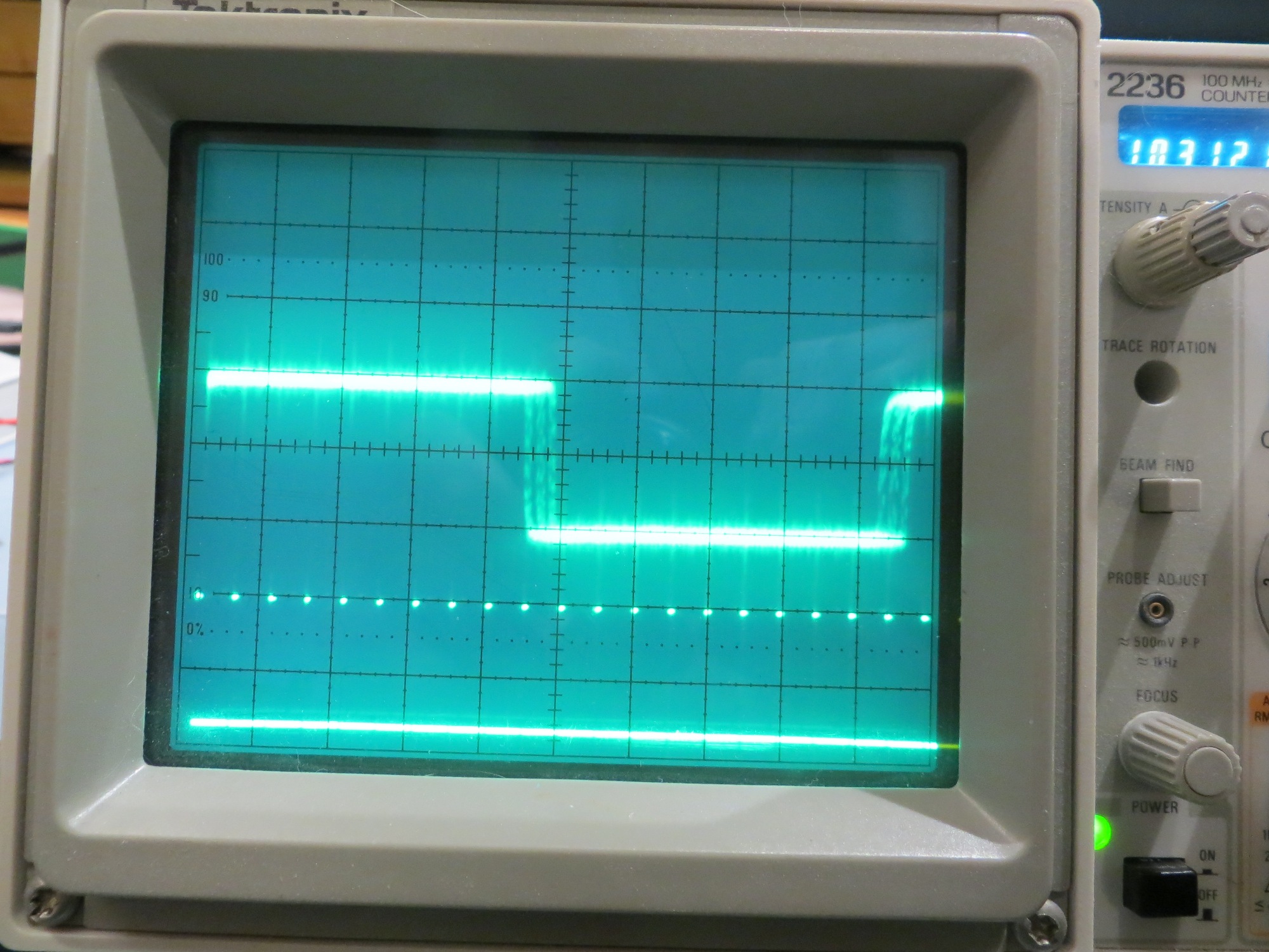
Output from Teensy 3.5 DAC0 (A21) pin
So, now I know that the DAC output works – now I just need to scale the ‘Final Value’ numbers correctly and connect them to the DAC output. Then I can watch the filter action in real time without worrying about the impact of print statements.
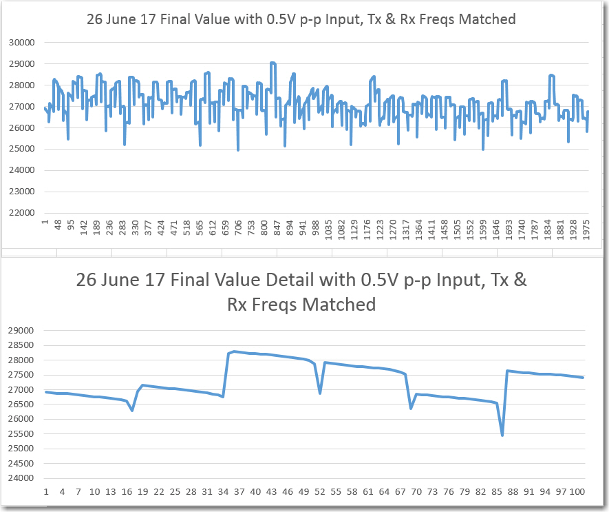
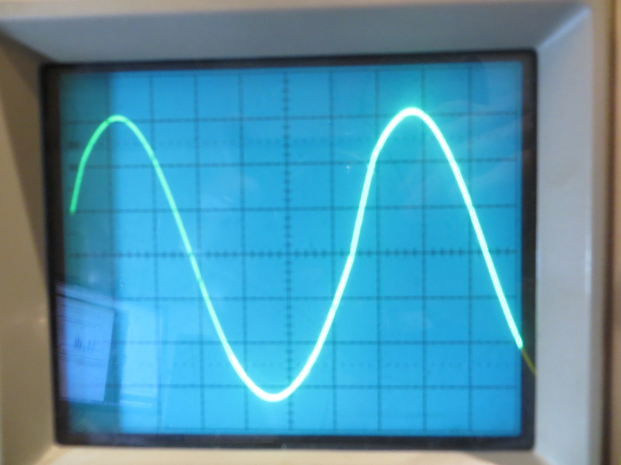
With an input square wave amplitude of about 0.35V p-p, or about 0.35/3.3 = 0.106 FS, the output is about 29,000. Therefore the peak output from the FV stage should be about 29,000/0.106 ~ 273,584. so an input of 0.35/3.3 = 0.106 should produce an output of (29,000/273584) *3.3 = 0.106*3.3 = 0.35
So, I modified my Sinewave test code to output the Final Value number, scaled by 273,584, and got the following display. In this test, the input amplitude is about 0.35V p-p, and the output is about 0.35VDC
Stay tuned,
Frank