Posted 15 November 2022
Last April I described how I determined that individual VL53L0X ‘time-of-flight’ distances sensors exhibited measurement errors, and also described my method for minimizing those errors. This has worked well up to now, but I recently realized that there was another error term I hadn’t accounted for; the error associated with using integer variables to hold VL53L0X distance measurements.
The left & right 3-element VL53L0X arrays (plus a single rear distance sensor) are managed by a dedicated Teensy 3.5 processor, which retrieves distance measurements from all seven sensors and then calibrates them using the method described in my April post. When requested by the main processor, these measurements (in integer MM) are provided via a I2C link. After receipt from the VL53L0X processor, distance measurements are converted from MM to CM by dividing by 10, ignoring integer truncation.
However, I have recently discovered that this integer truncation may well be more significant that I originally thought, and may be leading to performance issues, particularly with my ‘RotateToParallelOrientation()’ function and wall offset tracking in general. The linear distance between the front and rear VL53L0X sensor on each side is about 8.5Cm. Assuming that all constant errors are calibrated out, the robot will be parallel to the wall when the front and rear sensors return the same value. However, because the distance values only change in 1Cm increments, the actual distances measured by the front and rear sensors can be as much as 1Cm different. 1Cm difference over a length of 8.5Cm is about 7∘ – small, but not necessarily insignificant.
It turned out to be relatively painless to change all VL53L0X distance variables from ‘uint16_t’ to ‘float’, and get everything going again. After making this change I tried some more ‘rotate to parallel’ experiments but the change didn’t seem to make much of an improvement. Poking around a bit more I found out why – the raw measurement data coming from the VL53L0X sensors exhibited a lot of ‘noise’, even with the robot stationary and only a few cm from the nearby ‘wall’. The following Excel plot shows one sensor’s data with the robot approximately 14cm from the wall.
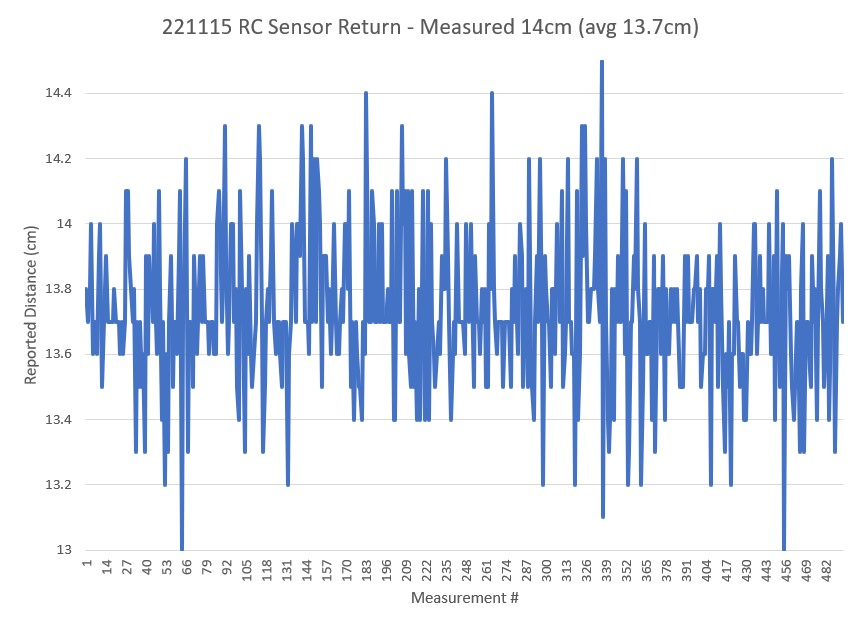
As can be seen from the above the reported distance varies from 13 to about 14.5cm. Assuming that all three right-hand sensors behave similarly, it would be possible for the front sensor to report 13cm while the rear sensor was reporting 14.5cm. Moreover, my parallel find algorithm defines ‘parallel’ as RF-RR ~= 0, so it can (and does) terminate well before or after the actual physical parallel orientation occurs.
Looking through (again) the VL53L0X documentation, I came across the ‘measurement budget’ parameter, which is set by default to ‘30000’ (30msec). In my application I had it set to ‘20000’ (20msec) because I thought at the time that with 7 total VL53L0X sensors, I couldn’t afford 30msec delay for each and still hold to a 200msec system loop period. I later changed the system design to use a separate Teensy 3.5 to continuously poll the sensors and report the latest measurement to the main processor when asked, which essentially eliminated the sensor delay from the overall loop (not entirely, as longer sensor measurement times may mean that physical dynamics aren’t followed quite as faithfully, but fortunately my robot doesn’t do anything quickly).
To test the effect of longer measurement budgets, I placed my robot in a cardboard box with its right-side sensor array about 7cm from the wall of the box, and then took measurements with measurement budgets of20, 30, 40, 50, and 60msec. For each value I plotted the distance output and also calculated the variance for each sensor, as shown in the plots below:
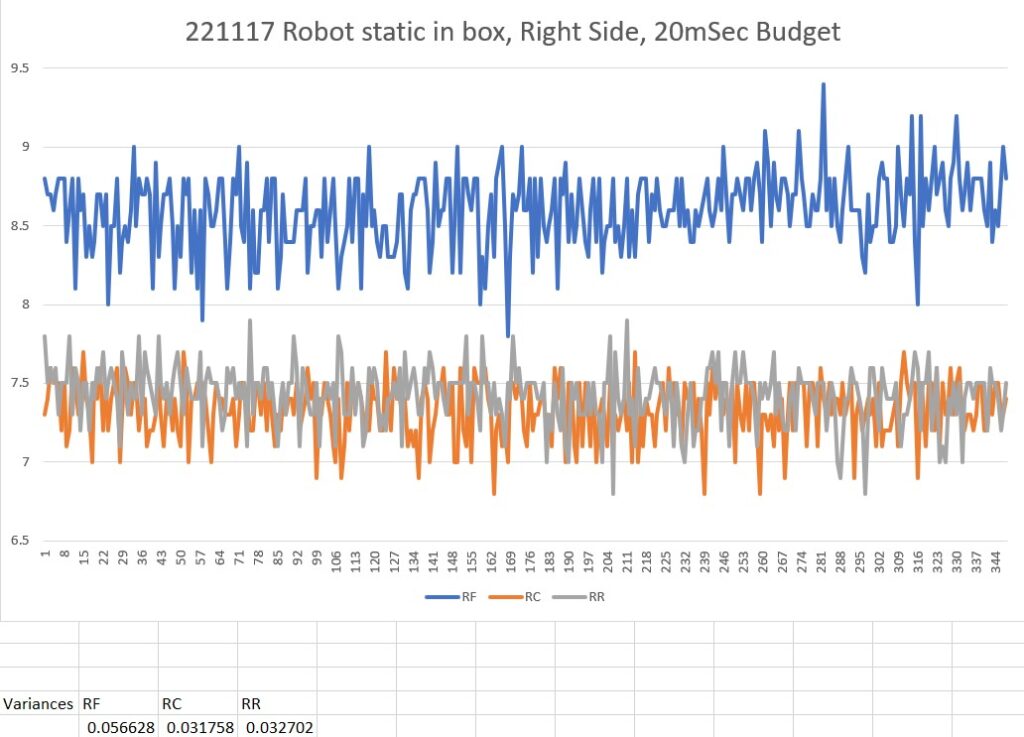
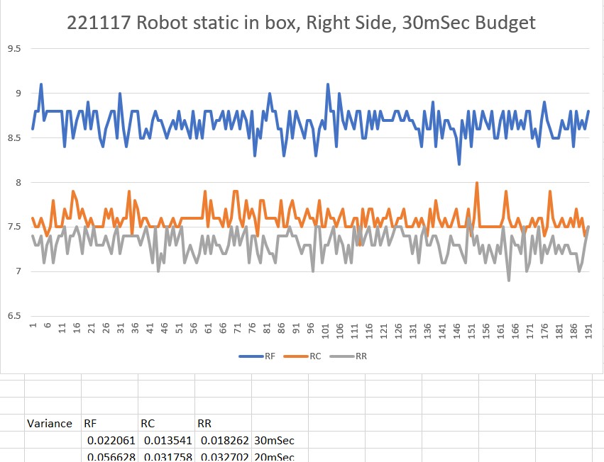
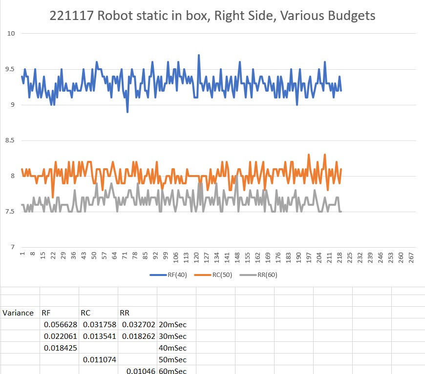
As can be seen from the chart immediately above, a measurement budget of 50msec is noticeably better than that for 40msec (which is itself better than the 20 or 30msec budgets), but the 60msec budget plot shows little improvement over 50msec. Looking The ‘RF’ variance starts at 0.0566 for 20msec, drops to less than half that at 30msec, drops by half again at 40msec, and drops by another 50% or so at 50msec. From there to 60msec is only a change from 0.011074 to 0.01046 (this all assumes that I can draw conclusions like this when not only going up with measurement budget, but going across sensors as well). In any case, I settled on a new measurement budge value of 50msec, as shown below.
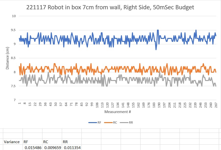
Note that while the motionless measurement variation has been significantly improved, I still have a problem with different nominal measurements from each sensor; the right-front (RF) sensor insists the wall is about 9.2cm away, while the center (RC) and rear (RR) ones think the wall is about 8 and 7.7cm away, respectively (as a side note, before I changed reported measurement variables from ‘uint_16’ to ‘float’, these values would have been reported as 9,8, and 7cm respectively). I thought I had fixed this problem earlier with a set of correction functions as described here, but I obviously have some more work to do (see this post for more on distance correction)
Stay tuned,
Frank
