Posted 19 June, 2017
In my last post on this subject, I showed that my 4-sensor band-pass filter (BPF) algorithm was feasible when run on a Teensy 3.5 SBC. However, what I haven’t done yet is to verify that the algorithm is indeed producing valid results, when fed with real sensor input.
I should be able to verify proper algorithm operation with my single-sensor test bed (as shown in the following photo) by moving the single sensor input line to each sensor channel (ADC input) in turn, and monitoring the data at different stages in the processing chain.
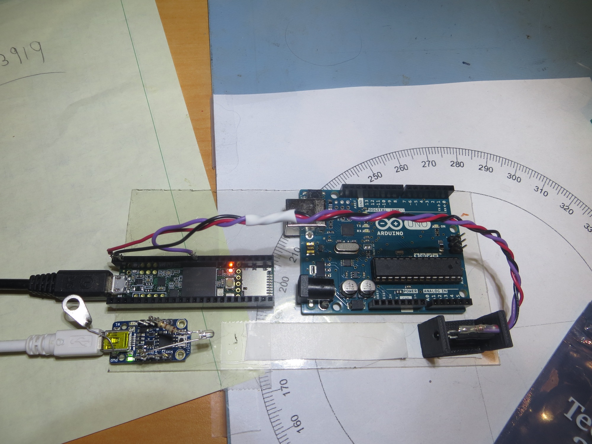
Teensy 3.5 installed on my algorithm test bed, with the Uno shown for size comparison. The small processor in the foreground is an Adafruit ‘Trinket’
Since I now have plenty of RAM to play with, I should be able to save a representative sample of the input data and intermediate results in suitably sized arrays, run the algorithm long enough to fill those arrays, and then print them all out at the end.
- I will probably want to run the process long enough to completely fill the 64-element I & Q ‘running sum’ arrays. These arrays already exist for all 4 sensor channels, so this has no effect on available RAM
- The next step backward in the chain are the I & Q ‘cycle group sum’ elements (one pair per sensor channel) used to generate one element in the running sum arrays. To store all these cycle group sum elements will require two 256-element arrays per sensor channel.
- And the first step in the process is the raw sensor input data. To store all the data required to generate 64 elements in the running sum arrays will require a single 1280-element array per sensor channel.
In summary, to instrument one sensor channel from start to finish will require
- 1ea 1280-element array to hold the raw data
- 2ea 256-element arrays to hold the cycle group sums
for a total of 1280 + 512 = 1796 elements at 2 bytes/element = 3592 bytes. If I wanted to do this for all 4 sensor channels at once, the total would be 14368 bytes, still well within the 192KB RAM availability on the Teensy – nice!
Results – Capture Stage:
The first step was to capture/display the raw ADC data to make sure that part was operating correctly. The plots below show all 4 sensor channels.
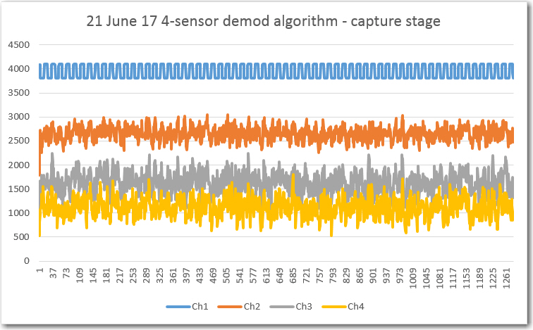
Raw ADC data for all 4 sensor channels, 1280 elements (enough to fill the entire 64-element running sum array)
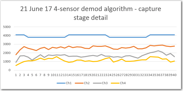
First 40 elements of the raw ADC capture
As can be seen in the above plots, channel 1 shows the 520Hz detected IR waveform, and the other three channels show just noise.
Results – Intermediate Stages:
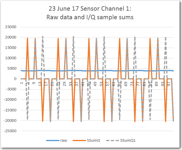
The next step was to verify proper operation of the step that accumulates a 1/4 cycle group of samples and generates the I & Q ‘sample group sum’ components. To verify this stage of the algorithm, I captured 5 cycles of data, as shown below:

Sensor channel 1 raw data and I/Q sample group sums
In the above plot, the dark blue line is the raw ADC data input, which varies from about the ADC maximum of 4096 to about 3890, or about 161mV (3.3V ADC reference and IR detector supply). The resulting ‘sample group sums’ are shown in orange (for the I component) and gray (for the Q component). The significance of the plot is that the sample group sums and the I/Q component generation appears to be happening correctly. The orange points follow a {+1, +1, -1, -1} sequence, while the gray ones follow a {+1, -1, -1, +1} sequence, as expected.
Next, I printed out this same 5-cycle segment in text form, as shown below (double-click in code window to enable scrollbar)
|
1 2 3 4 5 6 7 8 9 10 11 12 13 14 15 16 17 18 19 20 21 22 23 24 25 |
samp# raw SSumI1 SSumQ1 CSumI1 CSumQ1 0: 4094 0 0 1: 3893 0 0 2: 3895 0 0 3: 3895 0 0 4: 3896 19673 -19673 5: 3896 0 0 6: 3896 0 0 7: 3898 0 0 8: 3897 0 0 9: 3897 19484 19484 10: 4039 0 0 11: 4094 0 0 12: 4095 0 0 13: 4095 0 0 14: 4095 -20418 20418 15: 4095 0 0 16: 4095 0 0 17: 4095 0 0 18: 4095 0 0 19: 4095 -20475 -20475 -1736 -246 20: 3956 0 0 21: 3896 0 0 22: 3896 0 0 23: 3896 0 0 |
The above table shows the raw data, the sample-group sums, and the corresponding cycle-group sums. For example, the first set of 5 data samples adds to 19673. Since this is the first sample-group sum, it is multiplied by “+1” to form the I component, and “-1” to form the Q component, and these are shown adjacent to the last raw data in that sample group. After 4 such sample-group sums, the cycle-group sum I/Q components are generated by adding the 4 sample-group I/Q components respectively; for the first cycle these are -1736 & -246 as shown adjacent to the 20th sample (sample #19).
Results – Final Stages:
The cycle-sum I & Q components generated above are saved in separate 64-element circular buffers, and the running sum of these buffers are then used to form the final demodulated value for the channel of interest. The final value is computed as the sum of the absolute values of the I & Q component running sums, i.e. FV = abs(RunningSumI) + abs(RunningSumQ). To demonstrate proper algorithm functioning, I printed out the computed final values for well over 1000 cycles of raw data, as shown in the Excel plot below
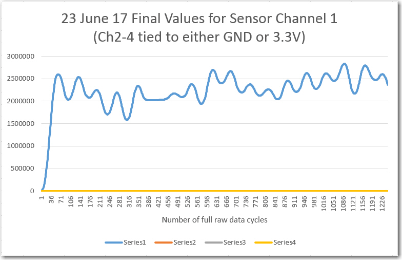
Computed final values vs complete input data cycles for sensor channel 1
As shown in the plot above, the final value rapidly rises from zero to around 2×10⁶ in the first 64 cycles of the run, after which it generally levels off for the rest of the run. There is quite a bit of ripple on the signal, which my friend and mentor John Jenkins mentioned might happen as the non phase-locked input and sampling frequencies slowly slid by each other (at least I hope that is what is happening!).
So, it looks like the algorithm is doing what it should, and my ‘scope measurements to date indicate that the Teensy is doing it all without breaking a sweat, even with print statements thrown in. It appears that I could probably double the number of samples/cycle and still have plenty of time to finish all the computations.
However, there are still a number of things to be accomplished before this new feature makes it into the field.
For starters, I’m not sure how to normalize the final value. For a fairly weak (~160mv out of 3V) signal the final value is north of 2 million – what happens for stronger signals, and how to I normalize this down to a range that I can use to drive an analog output? I suppose I could simply apply the IR modulation signal directly to the analog input (bypassing the IR path entirely) and see what happens, but I’d also like to understand the math. Maybe John Jenkins can help with this (hint, hint, wink, wink!).
Also, I’d like to validate the idea that this algorithm will selectively reject other signals that aren’t close to the desired 520Hz modulation frequency. I plan to test this by modifying the Trinket algorithm to make it a swept frequency generator (say from 470 – 570 Hz) and see how the output changes.
Stay tuned!
Frank
