Posted 15 October 2022
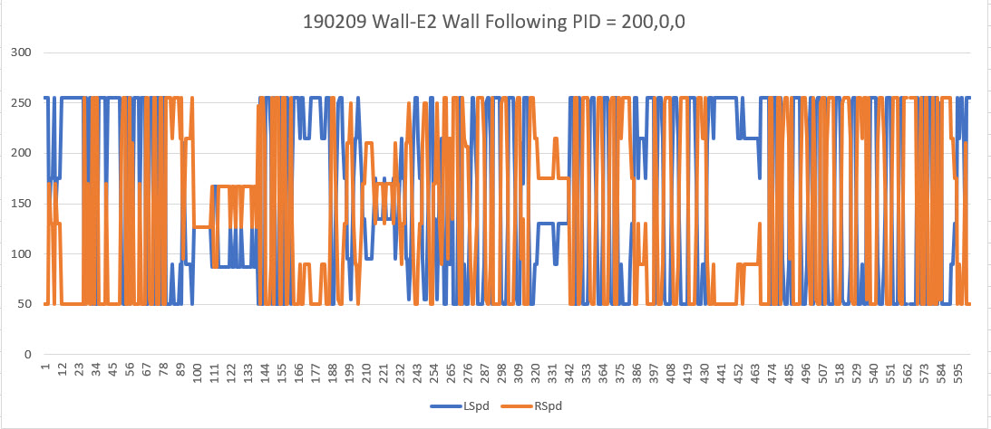
While working on my new ‘RunToDaylight’ algorithm for WallE3, my autonomous wall-following robot, I noticed that when WallE3 finds a wall to track after travelling in the direction of most front distance, it doesn’t do a very good job at all, oscillating crazily back and forth, and sometimes running head-first into the wall it is supposedly trying to track. This is somewhat disconcerting, as I thought I had long ago established a good wall tracking algorithm. So, I decided to once again plunge headlong into the swamps and jungles of my wall-tracking algorithm, hoping against hope that I won’t get eaten by mosquitos, snakes or crocodiles.
I went back to my latest part-task program, ‘WallE3_WallTrackTuning’. This program actually does OK when the robot starts out close to the wall, as the ‘CaptureWallOffset()’ routine is pretty effective. However, I noticed that when the robot starts out within +/- 4cm from the defined offset value, it isn’t terribly robust; the robot typically just goes straight with very few adjustments, even as it gets farther and farther away from the offset distance – oops!
So, I created yet another part-task program ‘WallE3_WallTrackTuning_V2’ to see if I could figure out why it isn’t working so well. With ‘WallE3_WallTrackTuning’ I simply called either TrackLeftWallOffset() or TrackRightWallOffset() and fed it the user-entered offset and PID values. However, this time I decided to pare down the code to the absolute minimum required to track a wall, as shown below (user input code not shown for clarity):
|
1 2 3 4 5 6 7 8 9 10 11 12 13 14 15 16 17 18 19 20 21 22 23 24 25 26 27 28 29 30 31 32 33 34 35 36 37 38 39 40 41 42 43 44 45 46 47 48 49 50 51 52 53 54 55 56 57 58 59 60 61 62 63 64 65 66 67 68 69 70 71 72 73 74 75 76 77 78 79 80 |
while (true) { //10/16/22 starting over with wall track tuning float kp = WallTrack_Kp; float ki = WallTrack_Ki; float kd = WallTrack_Kd; float lastError = 0; float lastInput = 0; float lastIval = 0; float lastDerror = 0; WallTrackSetPoint = OffCm; //04/17/22 this value holds robot parallel to left wall gl_pSerPort->printf("\nTrackLeftWallOffset: Start tracking offset of %2.1fcm with Kp/Ki/Kd = %2.2f\t%2.2f\t%2.2f\n", WallTrackSetPoint, kp, ki, kd); gl_pSerPort->printf(WallFollowTelemHdrStr); //Step4: Track the wall using PID algorithm mSecSinceLastWallTrackUpdate = 0; //added 09/04/21 MsecSinceLastFrontDistUpdate = 0; //added 10/02/22 to slow front LIDAR update rate while (true) { CheckForUserInput(); //this is a bit recursive, but should still work (I hope) if (mSecSinceLastWallTrackUpdate > WALL_TRACK_UPDATE_INTERVAL_MSEC) { mSecSinceLastWallTrackUpdate -= WALL_TRACK_UPDATE_INTERVAL_MSEC; //03/08/22 abstracted these calls to UpdateAllEnvironmentParameters() UpdateAllEnvironmentParameters();//03/08/22 added to consolidate sensor update calls //from Teensy_7VL53L0X_I2C_Slave_V3.ino: LeftSteeringVal = (LF_Dist_mm - LR_Dist_mm) / 100.f; //rev 06/21/20 see PPalace post float orientdeg = GetWallOrientDeg(glLeftSteeringVal); float orientrad = (PI / 180.f) * orientdeg; float orientcos = cosf(orientrad); glLeftCentCorrCm = glLeftCenterCm * orientcos; if (!isnan(glLeftCentCorrCm)) { //gl_pSerPort->printf("just before PIDCalcs call: WallTrackSetPoint = %2.2f\n", WallTrackSetPoint); WallTrackOutput = PIDCalcs(glLeftCentCorrCm, WallTrackSetPoint, lastError, lastInput, lastIval, lastDerror, kp, ki, kd); //04/05/22 have to use local var here, as result could be negative int16_t leftSpdnum = MOTOR_SPEED_QTR + WallTrackOutput; int16_t rightSpdnum = MOTOR_SPEED_QTR - WallTrackOutput; //04/05/22 Left/rightSpdnum can be negative here - watch out! rightSpdnum = (rightSpdnum <= MOTOR_SPEED_HALF) ? rightSpdnum : MOTOR_SPEED_HALF; //result can still be neg glRightspeednum = (rightSpdnum > 0) ? rightSpdnum : 0; //result here must be positive leftSpdnum = (leftSpdnum <= MOTOR_SPEED_HALF) ? leftSpdnum : MOTOR_SPEED_HALF;//result can still be neg glLeftspeednum = (leftSpdnum > 0) ? leftSpdnum : 0; //result here must be positive MoveAhead(glLeftspeednum, glRightspeednum); gl_pSerPort->printf(WallFollowTelemStr, millis(), glLeftFrontCm, glLeftCenterCm, glLeftRearCm, glLeftSteeringVal, orientdeg, orientcos, glLeftCentCorrCm, WallTrackSetPoint, lastError, WallTrackOutput, glLeftspeednum, glRightspeednum); } } } //09/29/22 if we get to here, hold in loop for user input mSecSinceLastWallTrackUpdate = 0; while (true) { CheckForUserInput(); if (mSecSinceLastWallTrackUpdate >= 10 * WALL_TRACK_UPDATE_INTERVAL_MSEC) { mSecSinceLastWallTrackUpdate -= 10 * WALL_TRACK_UPDATE_INTERVAL_MSEC; gl_pSerPort->printf("After exit from TrackRightWallOffset\n"); } } } |
The big change from previous versions was to go back to using the desired offset distance as the setpoint for the PID algorithm, and using the measured distance from the (left or right) center VL53L0X sensor as the input to be controlled. Now one might be excused from wondering why the heck I wasn’t doing this all along, as it does seem logical that if you want to control the robot’s distance from the near wall, you should use the desired distance as the setpoint and the measured distance as the input – duh!
Well, way back in the beginning of time, when I changed over from dual ultrasonic ‘Ping’ sensors to dual arrays of three VL53L0X LIDAR sensors well over 18 months ago, I wound up using a combination of the ‘steering value’ ( (front – rear)/100 ) and the reported center distance – desired offset as the input to the PID calc routine, as shown in the following code snippet:
|
1 2 3 4 5 6 7 8 9 10 11 12 13 14 15 16 17 18 19 20 21 22 23 24 25 26 27 28 29 30 31 32 33 34 35 36 37 38 39 40 41 42 43 44 45 |
while (true) { CheckForUserInput(); //this is a bit recursive, but should still work (I hope) //now using TIMER5 100 mSec interrupt for timing if (bTimeForNavUpdate) { //sinceLastComputeTime -= WALL_TRACK_UPDATE_INTERVAL_MSEC; bTimeForNavUpdate = false; //GetRequestedVL53l0xValues(VL53L0X_LEFT); //now done in TIMER5 ISR //have to weight value by both angle and wall offset WallTrackSteerVal = LeftSteeringVal + (Lidar_LeftCenter - 10 * WALL_OFFSET_TGTDIST_CM) / 1000.f; //update motor speeds, skipping bad values if (!isnan(WallTrackSteerVal)) { //10/12/20 now this executes every time, with interval controlled by timer ISR PIDCalcs(WallTrackSteerVal, WallTrackSetPoint, TIMER5_INTERVAL_MSEC, lastError, lastInput, lastIval, lastDerror, kp, ki, kd, WallTrackOutput); //PIDCalcs(WallTrackSteerVal, WallTrackSetPoint, WALL_TRACK_UPDATE_INTERVAL_MSEC, lastError, lastInput, lastIval, lastDerror, // kp, ki, kd, WallTrackOutput); int speed = 0; int leftspeednum = MOTOR_SPEED_QTR + WallTrackOutput; int rightspeednum = MOTOR_SPEED_QTR - WallTrackOutput; rightspeednum = (rightspeednum <= MOTOR_SPEED_FULL) ? rightspeednum : MOTOR_SPEED_FULL; rightspeednum = (rightspeednum > 0) ? rightspeednum : 0; leftspeednum = (leftspeednum <= MOTOR_SPEED_FULL) ? leftspeednum : MOTOR_SPEED_FULL; leftspeednum = (leftspeednum > 0) ? leftspeednum : 0; MoveAhead(leftspeednum, rightspeednum); mySerial.printf("%lu \t%d\t%d\t%d \t%2.2f\t%2.2f\t%2.2f\t%2.2f \t%2.2f\t%2.2f\t%2.2f \t%2.2f\t%d\t%d\n", millis(), Lidar_LeftFront, Lidar_LeftCenter, Lidar_LeftRear, WallTrackSteerVal, WallTrackSetPoint, lastError, lastIval, kp * lastError, ki * lastIval, kd * lastDerror, WallTrackOutput, leftspeednum, rightspeednum); } } } |
This is the line that calculates the input value to the PID:
|
1 2 |
//have to weight value by both angle and wall offset WallTrackSteerVal = LeftSteeringVal + (Lidar_LeftCenter - 10 * WALL_OFFSET_TGTDIST_CM) / 1000.f; |
This actually worked pretty well, but as I discovered recently, it is very difficult to integrate two very different physical mechanisms in the same calculations – almost literally oranges and apples. When the offset is small, the steering value term dominates and the robot simply continues more or less – but not quite – parallel to the wall, meaning that it slowly diverges from the desired offset – getting closer or further away. When the divergence gets large enough the offset term dominates and the robot turns toward the desired offset, but it is almost impossible to get PID terms that are large enough to actually make corrections without being so large as to cause wild oscillations.
The above problem didn’t really come to a head until just recently when I started having problems with tracking where the robot started off at or close to the desired offset value and generally parallel, meaning both terms in the above expression were near zero – for this case the behavior was a bit erratic to say the least.
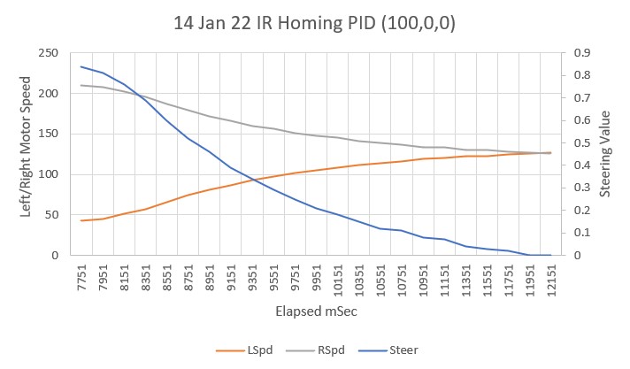
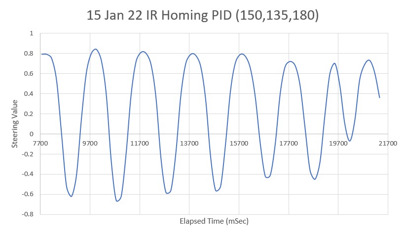
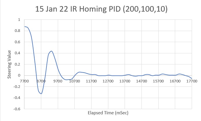
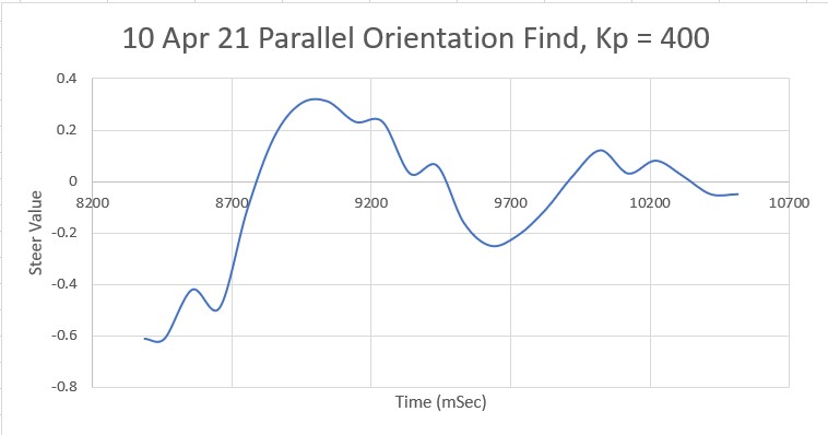
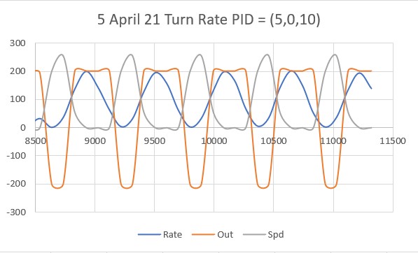
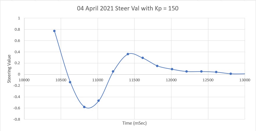
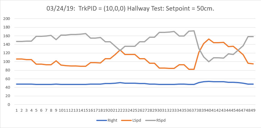
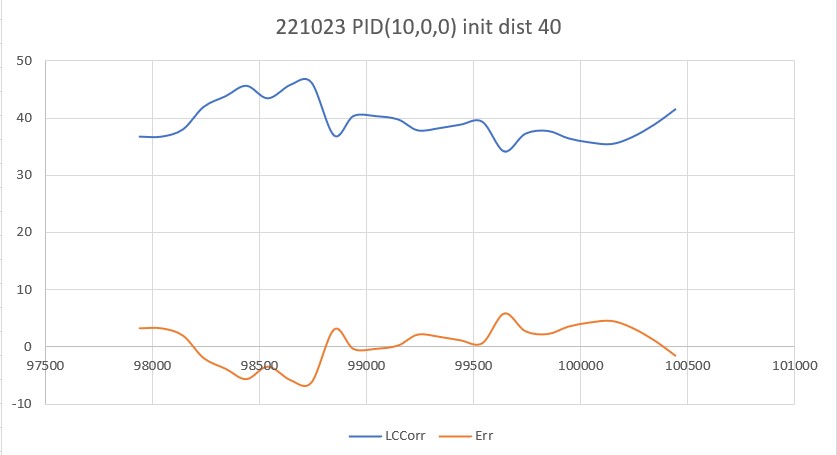
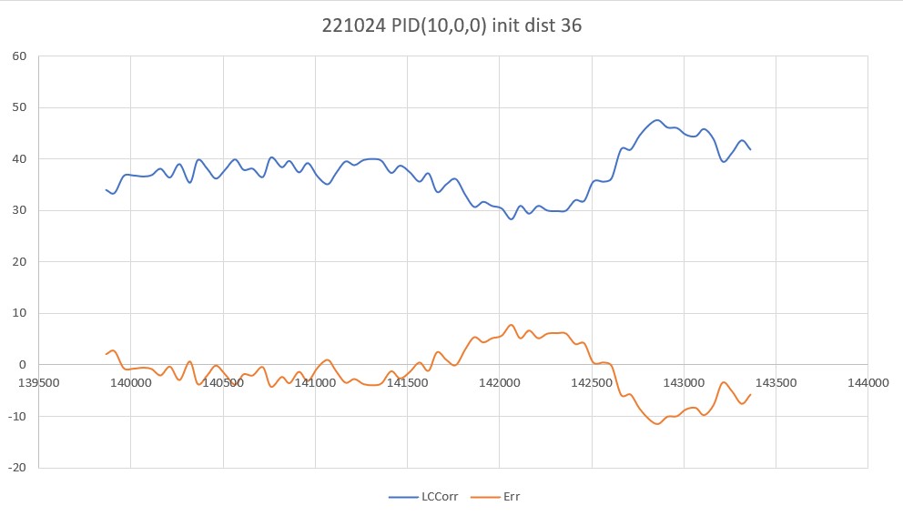
So, back to the basics. The following plot and short video show the robot’s behavior with the new setup (offset = 40cm, PID = (10,0,0)):
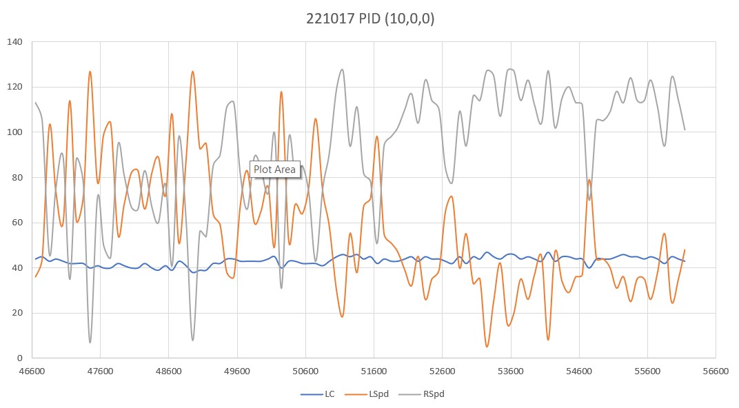
With this setup, the robot tracks the desired 40cm offset very well (average of 41.77cm), with a very slow oscillation. I’m sure I can tweak this up a bit with a slightly higher ‘P’ value and then adding a small amount of ‘I’, but even with the most basic parameter set the system is obviously stable.
20 October 2022 Update:
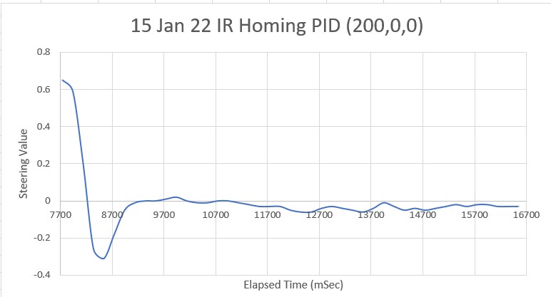
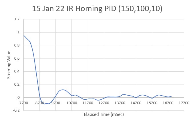
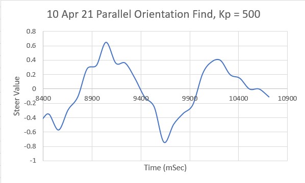
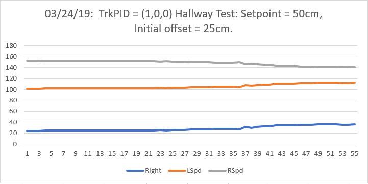
I made another run with PID(10,0,0), but this time I started the run with the robot displaced about 7cm from the 40cm offset. As shown in the plot and short video, this caused quite a large oscillation; not quite disastrous, but probably would have been if my test wall had been any longer.
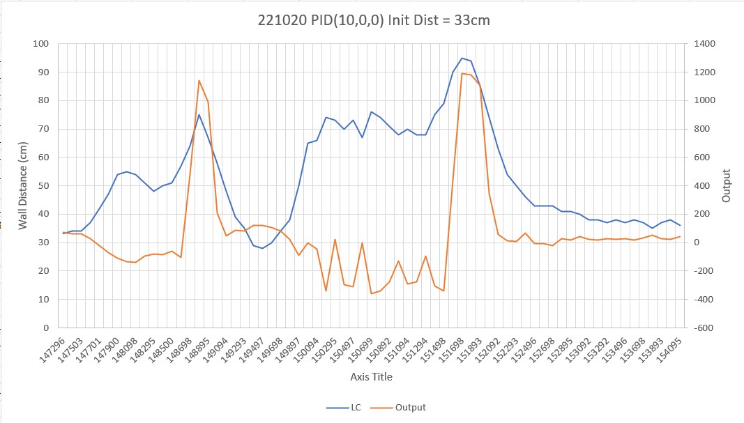
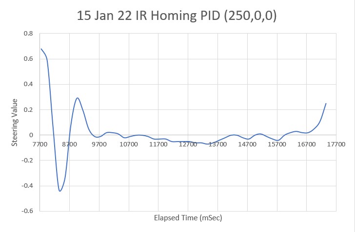
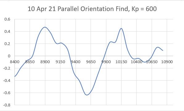
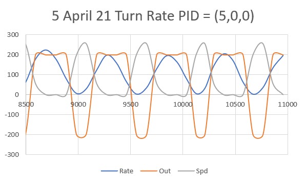
After looking at the data from this run, I decided to try lowering the P value from 10 to 5, thinking that the lower value would reduce the oscillation magnitude with a non-zero initial displacement from the desired setpoint. As the following plot and short video shows, the result was much better.
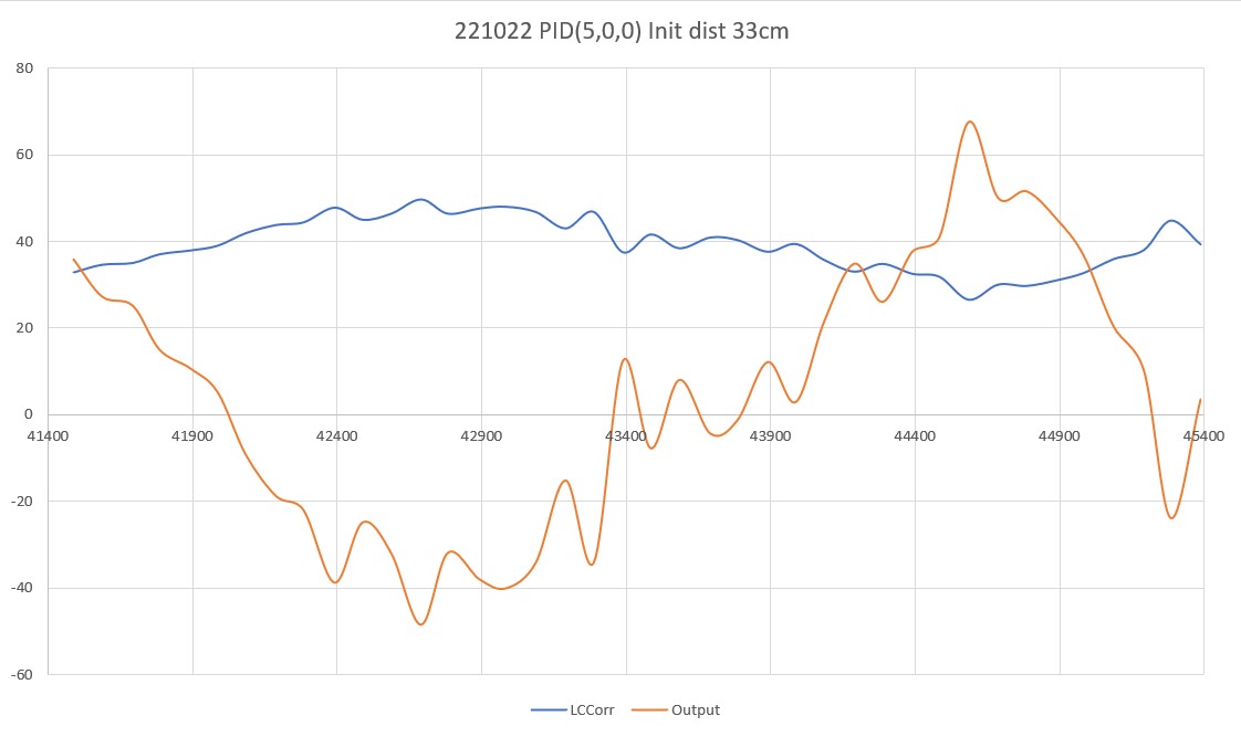
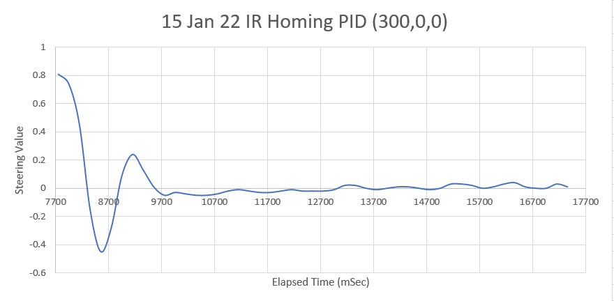
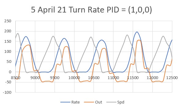
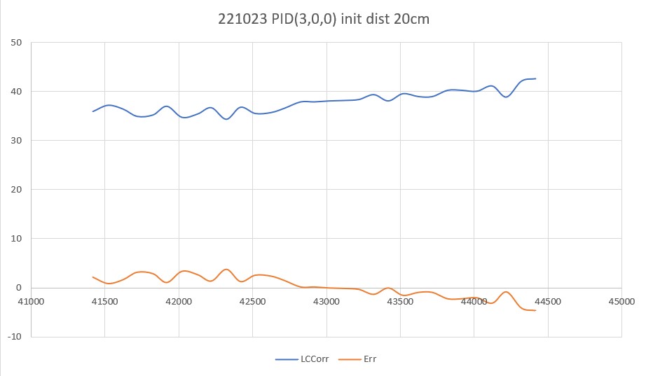
So then I tried PID(3,0,0), again with an initial placement of 33cm from the wall, 7cm from the setpoint of 40cm
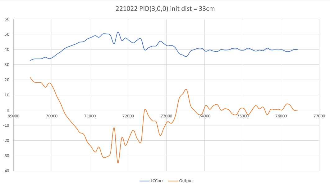
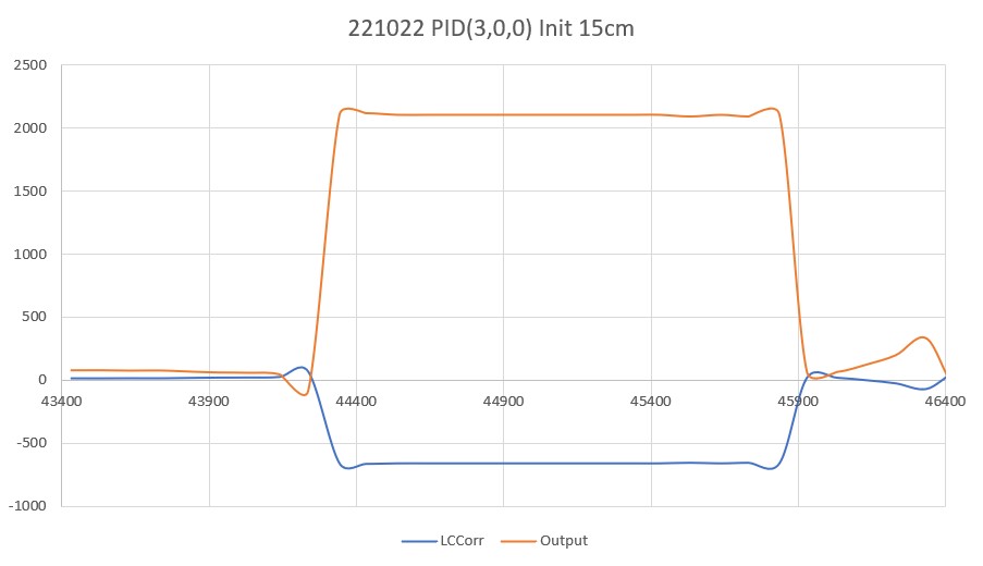
As shown by the plot and video, PID(3,0,0) does a very good job of recovering from the large initial offset and then maintaining the desired 40cm offset. This result makes me start to wonder if my separate ‘Approach and Capture’ stage is required at all. However, a subsequent run with PID (3,0,0) but with an initial placement of 15cm (25cm error) disabused me of any thoughts like that!
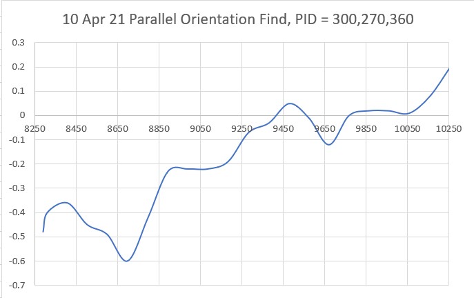
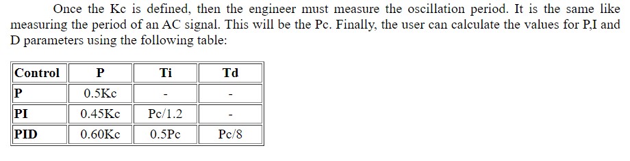
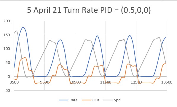
After talking this over with my PID-expert stepson, he recommended that I continue to decrease the ‘P’ term until the robot never quite gets to the desired setpoint before running out of room, and then adding some (possibly very small) amount of ‘D’ to hasten capture of the desired setpoint. So, I continued, starting with a ‘P’ value of 2, as shown below:
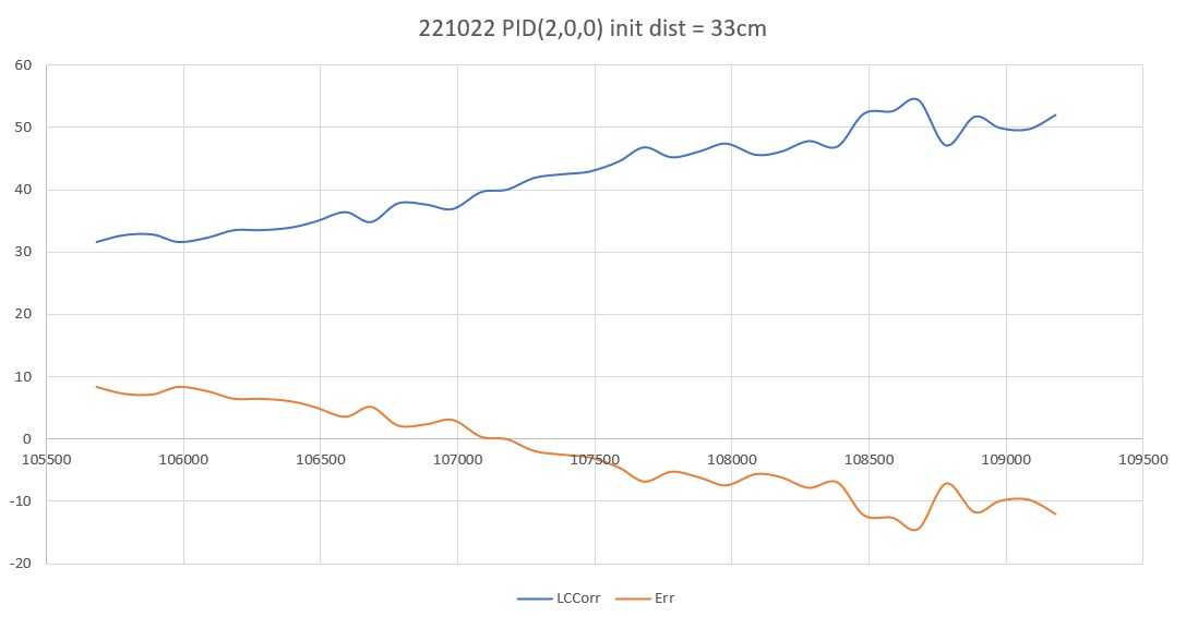
This result was a bit unexpected, as I thought such a ‘straight-line’ trajectory should have ended before going past the 40cm setpoint, indicating that I had achieved my ‘not quite controlling’ value of ‘P’. However, after thinking about a bit and looking at the actual data (shown below), I think what this shows is that the robot case is fundamentally different than most PID control applications in that reducing the error term (and thus the ‘drive’ signal) doesn’t necessarily change the robot’s trajectory, as the robot will tend to travel in a straight line in the absence of a contravening error term. In other words, removing the ‘drive’ due to the error term doesn’t cause the robot to slow down, as it would in a normal motor drive scenario.
|
1 2 3 4 5 6 7 8 9 10 11 12 13 14 15 16 17 18 19 20 21 22 23 24 25 26 27 28 29 30 31 32 33 34 35 36 37 |
Msec LF LC LR Steer Deg Cos LCCorr Set Err Output LSpd RSpd 105681 31 33 33 -0.28 -16 0.96 31.7 40 8.3 16.6 91 58 105781 30 33 32 -0.12 -6.86 0.99 32.8 40 7.2 14.5 89 60 105886 31 33 32 -0.07 -4 1 32.9 40 7.1 14.2 89 60 105980 31 33 34 -0.28 -16 0.96 31.7 40 8.3 16.6 91 58 106087 31 33 33 -0.19 -10.86 0.98 32.4 40 7.6 15.2 90 59 106182 32 34 33 -0.16 -9.14 0.99 33.6 40 6.4 12.9 87 62 106280 32 34 34 -0.16 -9.14 0.99 33.6 40 6.4 12.9 87 62 106388 33 34 33 -0.04 -2.29 1 34 40 6 12.1 87 62 106482 33 35 34 -0.04 -2.29 1 35 40 5 10.1 85 64 106589 34 37 36 -0.16 -9.14 0.99 36.5 40 3.5 6.9 81 68 106683 35 35 36 -0.07 -4 1 34.9 40 5.1 10.2 85 64 106781 36 38 36 -0.08 -4.57 1 37.9 40 2.1 4.2 79 70 106885 36 39 38 -0.26 -14.86 0.97 37.7 40 2.3 4.6 79 70 106981 37 38 39 -0.23 -13.14 0.97 37 40 3 6 80 69 107084 38 40 39 -0.12 -6.86 0.99 39.7 40 0.3 0.6 75 74 107179 38 42 41 -0.3 -17.14 0.96 40.1 40 -0.1 -0.3 74 75 107279 39 43 41 -0.22 -12.57 0.98 42 40 -2 -3.9 71 78 107388 40 43 41 -0.14 -8 0.99 42.6 40 -2.6 -5.2 69 80 107479 42 43 42 -0.03 -1.71 1 43 40 -3 -6 69 80 107586 42 46 44 -0.25 -14.29 0.97 44.6 40 -4.6 -9.2 65 84 107680 45 47 45 0.05 2.86 1 46.9 40 -6.9 -13.9 61 88 107780 44 49 47 -0.39 -22.29 0.93 45.3 40 -5.3 -10.7 64 85 107886 45 48 48 -0.27 -15.43 0.96 46.3 40 -6.3 -12.5 62 87 107979 47 49 50 -0.25 -14.29 0.97 47.5 40 -7.5 -15 60 89 108086 48 48 50 -0.31 -17.71 0.95 45.7 40 -5.7 -11.4 63 86 108179 48 49 51 -0.34 -19.43 0.94 46.2 40 -6.2 -12.4 62 87 108280 48 51 52 -0.35 -20 0.94 47.9 40 -7.9 -15.8 59 90 108384 49 50 53 -0.35 -20 0.94 47 40 -7 -14 61 88 108481 50 53 52 -0.16 -9.14 0.99 52.3 40 -12.3 -24.7 50 99 108586 51 53 52 -0.11 -6.29 0.99 52.7 40 -12.7 -25.4 49 100 108680 52 55 53 -0.13 -7.43 0.99 54.5 40 -14.5 -29.1 45 104 108781 50 54 55 -0.51 -29.14 0.87 47.2 40 -7.2 -14.3 60 89 108885 50 53 53 -0.21 -12 0.98 51.8 40 -11.8 -23.7 51 98 108978 52 55 56 -0.43 -24.57 0.91 50 40 -10 -20 54 95 109083 52 54 56 -0.4 -22.86 0.92 49.8 40 -9.8 -19.5 55 94 109181 52 54 55 -0.27 -15.43 0.96 52.1 40 -12.1 -24.1 50 99 |
23 October 2022 Update:
In previous work on this subject, I had already recognized that the ‘capture’ and ‘track’ phases of Wall-E’s behavior required separate treatment, and had implemented this with a ‘CaptureWallOffset()’ function to handle the ‘capture’ phase. This function calculates the amount of rotation needed to achieve an approximately 30 deg orientation angle with respect to the near wall, then moves forward to the desired wall offset value, and then turns back to parallel the near wall.
So, my next step is to re-integrate this ‘CaptureWallOffset()’ routine with my current distance-only based offset tracking algorithm. The idea is to essentially eliminate the problem space where the distance-only PID algorithm fails, so the PID only has to handle initial conditions very near the desired setpoint. When the ‘CaptureWallOffset()’ routine completes, the robot should be oriented parallel to the wall, and at a distance close to (but not necessarily the same as) the desired setpoint. Based on the above results, I think I will change the setpoint from the current constant value (40 cm at present) to match the measured distance from the wall at the point of ‘CaptureWallOffset()’ routine completion. This will guarantee that the PID starts out with the input matching the setpoint – i.e. zero error.
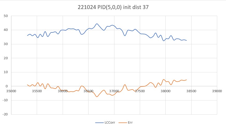
With this new setup, I made a run with the robot starting just 13cm from the wall. The CaptureWallOffset() routine moved the robot from the initial 13cm to about 37cm, with the robot ending up nearly parallel. The PID tracking algorithm started with an initial error term of +3.3, and tracked very well with a ‘P’ value of 10. See the plot and short video below. The video shows both the capture and track phases, but the plot only shows the track portion of the run.
Here’s a run with PID(3,0,0), starting at an offset of 22cm.
24 October 2022 Update:
While reading through some more PID theory/practice articles, I was once again reminded that smaller time intervals generally produce better results, and that struck a bit of a chord. Some time back I settled on a time interval of about 200mSec, but while I was working with my ‘WallTrackTuning_V2’ program I realized that this interval was due to the time required by the PulsedLight LIDAR to produce a front distance measurement. I discovered this when I tried to reduce the overall update time from 200 to 100mSec and got lots of errors from GetFrontDistCm(). After figuring this out, I modified the code to use a 200mSec time interval for the front LIDAR, and 100mSec for the VL53L0X side distance sensors.
So, it occurred to me that I might be able to reduce the side measurement interval even further, so I instrumented the robot to toggle a digital output (I borrowed the output for the red laser pointer) at the start and end of the wall tracking adjustment cycle, as shown in the code snippet below:
|
1 2 3 4 5 6 7 8 9 10 11 12 13 14 15 16 17 18 19 20 21 22 23 24 25 26 27 28 29 30 31 32 33 34 35 36 37 38 39 |
if (mSecSinceLastWallTrackUpdate > WALL_TRACK_UPDATE_INTERVAL_MSEC) { digitalToggle(RED_LASER_DIODE_PIN); //10/24/22 toggle duration measurement pulse mSecSinceLastWallTrackUpdate -= WALL_TRACK_UPDATE_INTERVAL_MSEC; //03/08/22 abstracted these calls to UpdateAllEnvironmentParameters() UpdateAllEnvironmentParameters();//03/08/22 added to consolidate sensor update calls //from Teensy_7VL53L0X_I2C_Slave_V3.ino: LeftSteeringVal = (LF_Dist_mm - LR_Dist_mm) / 100.f; //rev 06/21/20 see PPalace post float orientdeg = GetWallOrientDeg(glLeftSteeringVal); float orientrad = (PI / 180.f) * orientdeg; float orientcos = cosf(orientrad); glLeftCentCorrCm = glLeftCenterCm * orientcos; if (!isnan(glLeftCentCorrCm)) { //gl_pSerPort->printf("just before PIDCalcs call: WallTrackSetPoint = %2.2f\n", WallTrackSetPoint); WallTrackOutput = PIDCalcs(glLeftCentCorrCm, WallTrackSetPoint, lastError, lastInput, lastIval, lastDerror, kp, ki, kd); //04/05/22 have to use local var here, as result could be negative int16_t leftSpdnum = MOTOR_SPEED_QTR + WallTrackOutput; int16_t rightSpdnum = MOTOR_SPEED_QTR - WallTrackOutput; //04/05/22 Left/rightSpdnum can be negative here - watch out! rightSpdnum = (rightSpdnum <= MOTOR_SPEED_HALF) ? rightSpdnum : MOTOR_SPEED_HALF; //result can still be neg glRightspeednum = (rightSpdnum > 0) ? rightSpdnum : 0; //result here must be positive leftSpdnum = (leftSpdnum <= MOTOR_SPEED_HALF) ? leftSpdnum : MOTOR_SPEED_HALF;//result can still be neg glLeftspeednum = (leftSpdnum > 0) ? leftSpdnum : 0; //result here must be positive MoveAhead(glLeftspeednum, glRightspeednum); gl_pSerPort->printf(WallFollowTelemStr, millis(), glLeftFrontCm, glLeftCenterCm, glLeftRearCm, glLeftSteeringVal, orientdeg, orientcos, glLeftCentCorrCm, WallTrackSetPoint, lastError, WallTrackOutput, glLeftspeednum, glRightspeednum); } digitalToggle(RED_LASER_DIODE_PIN); //10/24/22 toggle duration measurement pulse |
Using my handy-dandy Hanmatek DSO, I was able to capture the pin activity, as shown in the following plot:
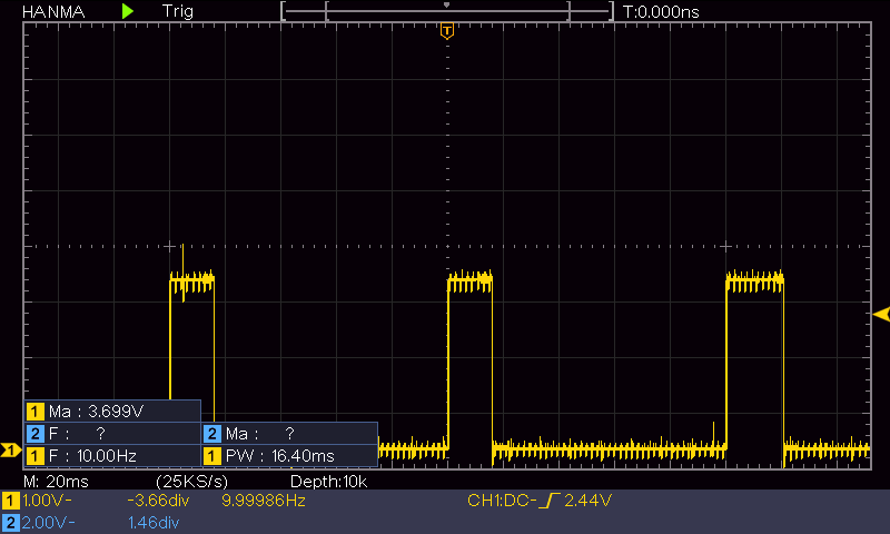
As shown above, the update code takes a bit less than 20mSec to complete, and idles for the remaining 80mSec or so, waiting for the 100mSec time period to elapse. So, I should be able to reduce the time interval by at least a factor of two. I changed the update interval from 100mSec to 50mSec, and got the activity plot shown below:
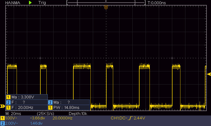
The above plot has the same 20mSec/div time scale as the previous one; as can be seen, there is still plenty of ‘idle’ time between wall tracking updates. Now to see if this actually changes the robot’s behavior.
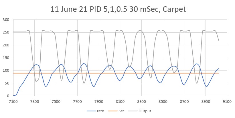
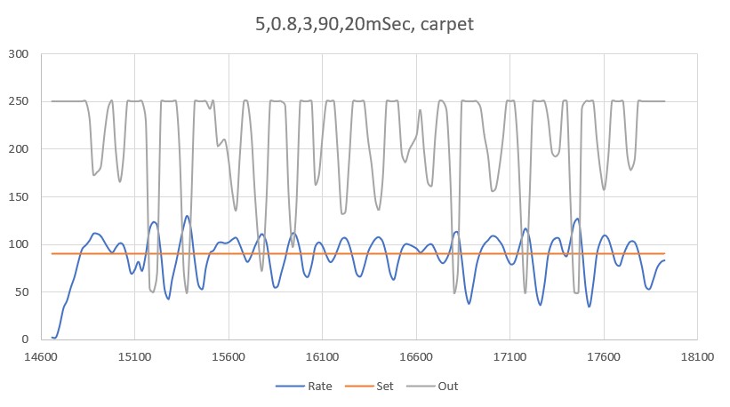
As shown in the next plot and video, I ran another ‘sandbox’ test, this time with the update interval set to 50mSec vice 100mSec, and with an 11Cm initial offset.
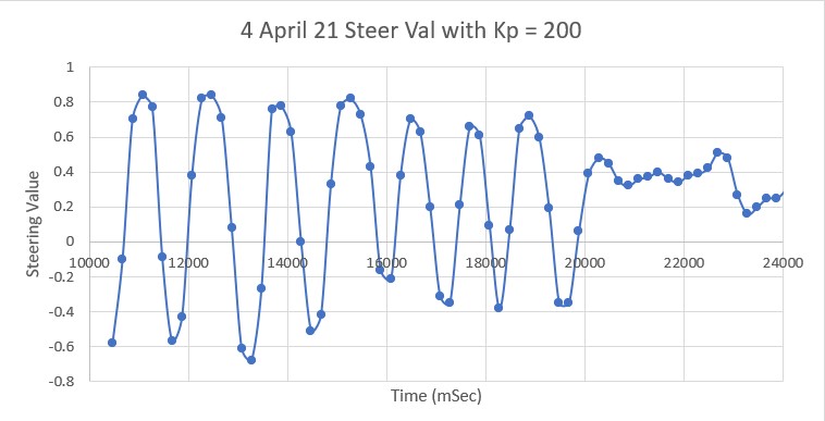
Then I ran it again, except this time with a PID of (10,0,0):
This wasn’t at all what I expected. I thought the larger ‘P’ value would cause the robot to more closely track the desired offset, but that isn’t what happened. Everything is fine for the first two seconds (140,000 to 142,000 mSec), but then the robot starts weaving dramatically- to the point where the motor values max out at 127 on one side and 0 on the other – bummer. Looks like I need another consulting session with my PID wizard stepson!
25 October 2022 Update:
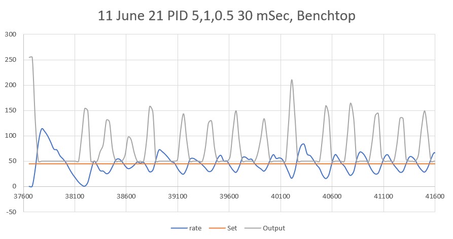
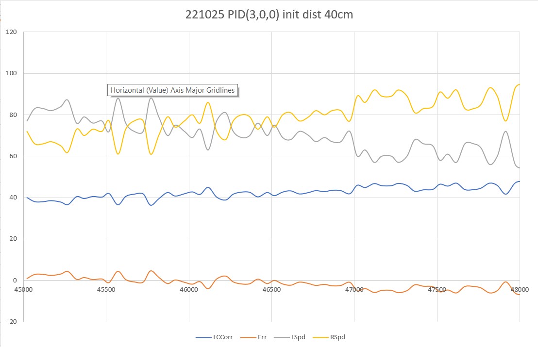
My PID wiz stepson liked my idea of breaking the wall tracking problem into an offset capture phase, followed by a wall tracking phase, but wasn’t particularly impressed with my thinking about reducing the PID update interval while simultaneously increasing the P value to 10, so, I’m back to taking more data. The following run is just the wall tracking phase, with 50mSec update interval and a P value of 3.
As can be seen, the robot doesn’t really make any corrections – just goes in a straight line more or less. However, the left/right wheel speed data does show the correct trend (left wheel drive decreasing, right wheel drive increasing), so maybe a non-zero ‘I’ value would do the trick?
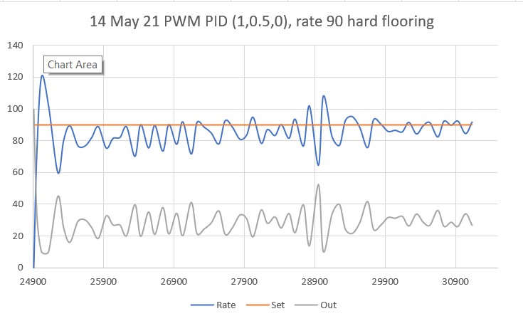
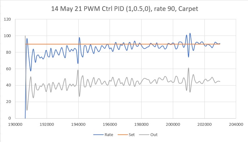
Here’s a run with PID(3,0.5,0):
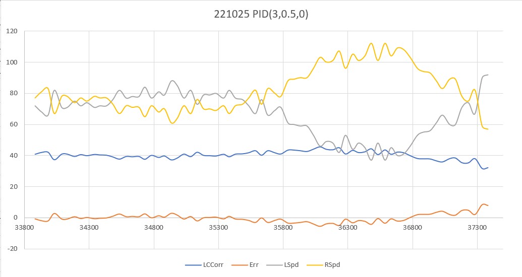
In the above plot the I value does indeed cause the robot to track back to the target distance, but then goes well past the target before starting to turn back. Too much I?
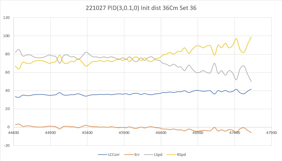
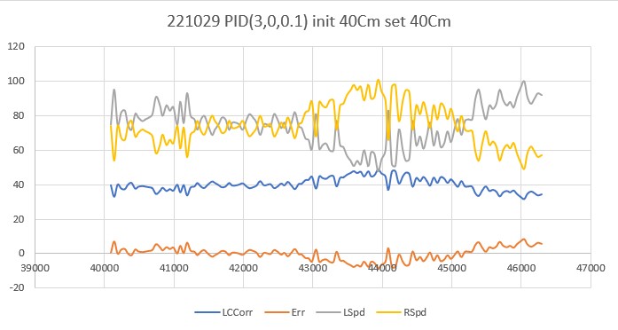
Here’s another run with PID(3,0.1,0) – looking pretty good!
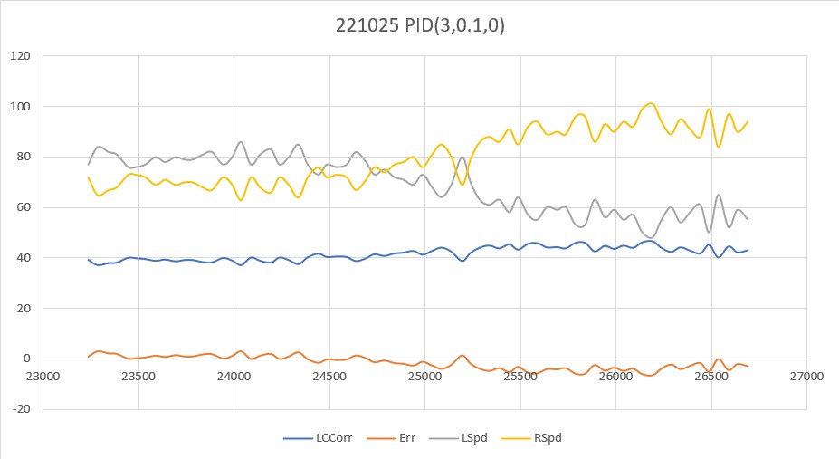
This looks pretty good; with I = 0.1 the robot definitely adjusted back toward the target distance, but in a much smoother manner than with I = 0.5. OK, time to let the master view these results and see if I’m even in the right PID universe.
One thing to mention in these runs – they are performed in my office, and the total run length is a little over 2m (210Cm), so I’m only seeing just one correction maneuver. Maybe if I start out with a small offset from the target value? Nope – that won’t work – at least not tonight; my current code changes the setpoint from the entered value (40Cm in this case) to the actual offset value (36Cm on this run) before starting the run. Curses! Foiled again!
27 October 2022 Update:
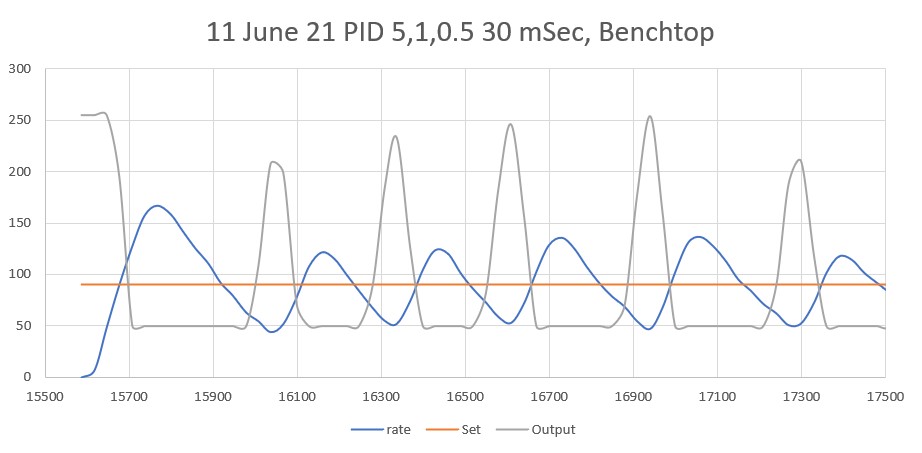
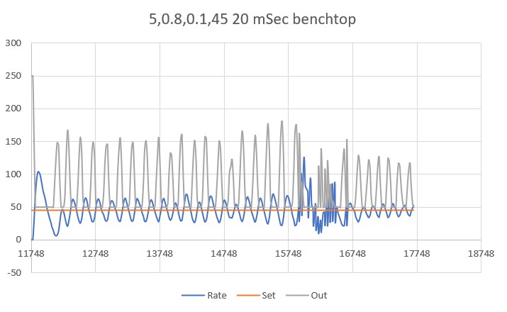
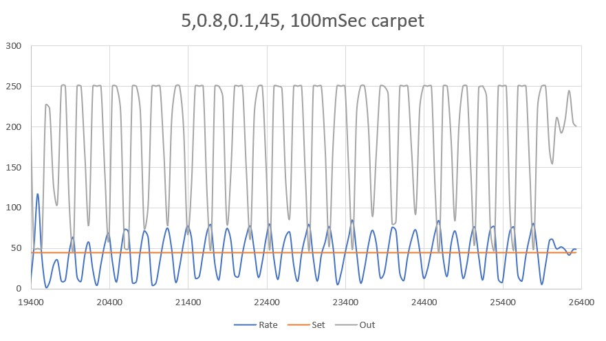
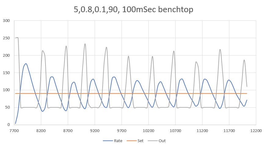
Today I had some time to see how the PID handles wall-tracking runs starting with a small offset from the desired value. First I started with a run essentially identical to the last run from two days ago, just to make sure nothing significant had changed (shouldn’t, but who knows for sure), as shown below:
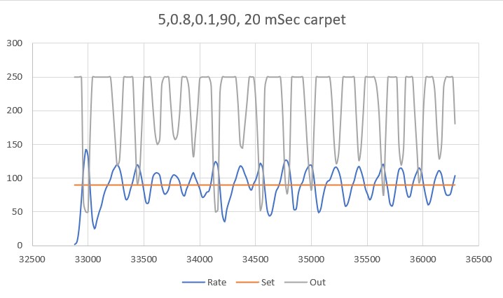
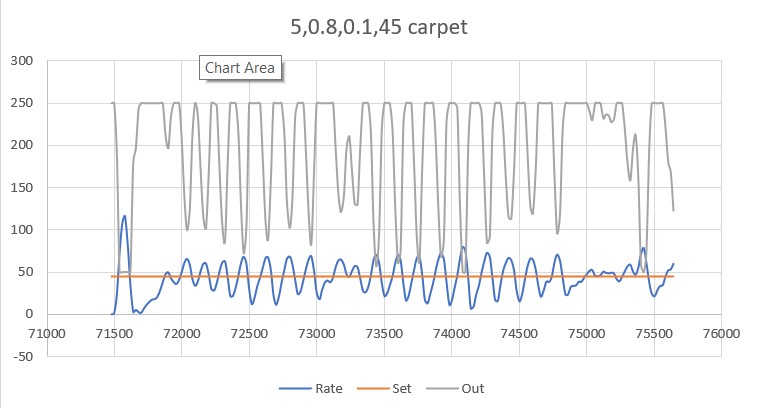
Then I tried a run with the same PID values, but with a small initial offset from the desired 40Cm:
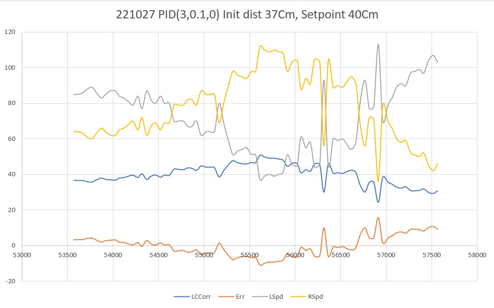
As can be seen, the robot didn’t seem to handle this very well; there was an initial correction away from the wall (toward the desired offset), but the robot cruised well past the setpoint before correcting back toward the wall. This same behavior repeated when the robot went past the setpoint on the way back toward the wall.
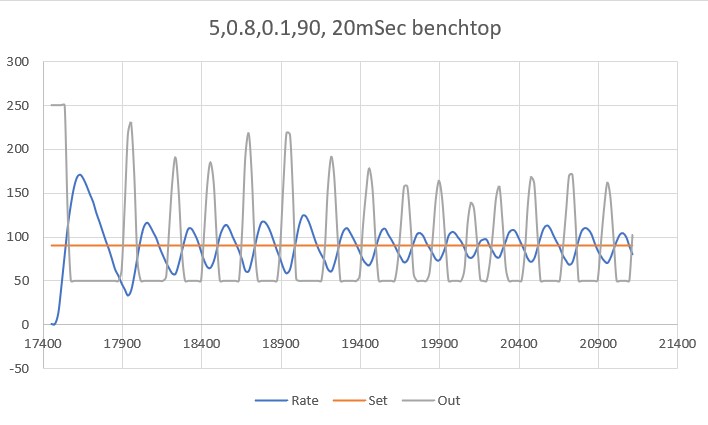
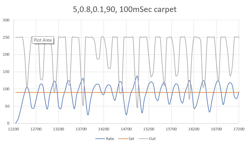
To see which way I needed to move with the ‘I’ value, a made another run with the ‘I’ value changed from 0.1 to 0.25, as shown below:
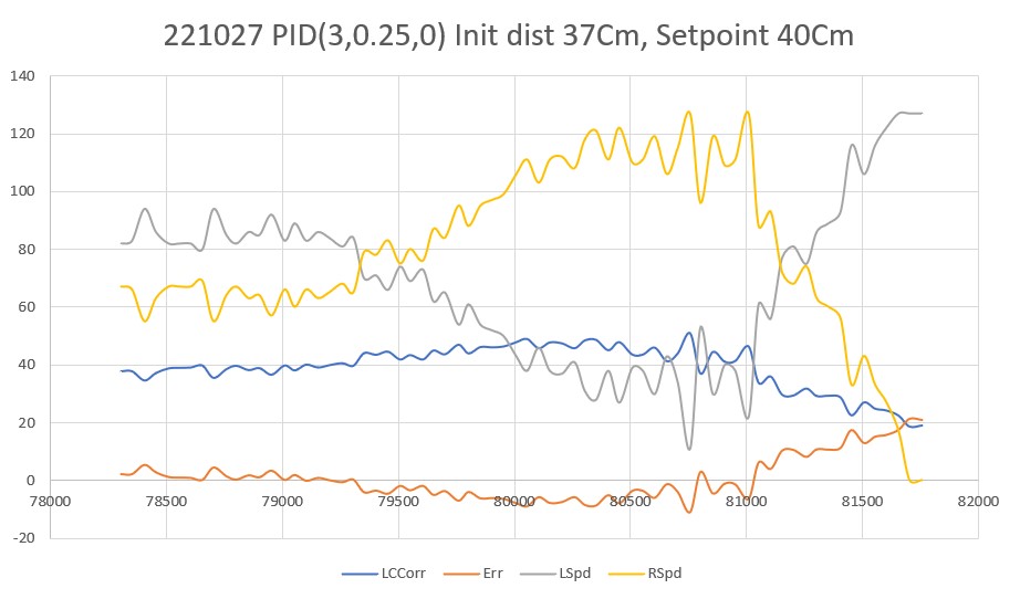
Now the corrections were much more dramatic, and tracking was much less accurate. on the second correction (when the robot passed through the desired setpoint going away from the wall), the motor drive values maxed out (127 on the left, 0 on the right).
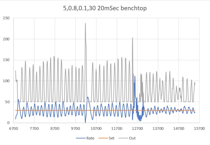
Next I tried an ‘I’ value of 0.05, as shown below:
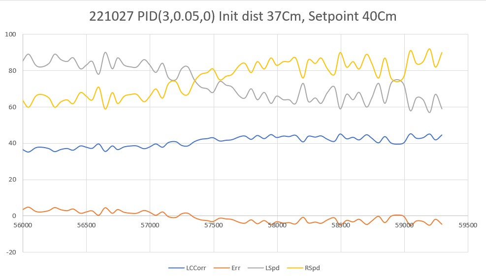
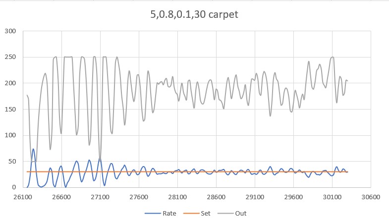
This looks much nicer – deviations from the desired offset are much smaller, and everything is much smoother. However, I’m a little reluctant to declare victory here, as it may well be that the ‘I’ value is so small now that it may not be making any difference at all, and what I’m seeing is just the natural straight-line behavior of the robot. In addition, the robot may not be able to track the wall around some of the 45deg wall direction changes found in this house.
28 October 2022 Update:
I decided to rearrange my office ‘sandbox’ to provide additional running room for my wall-following robot. By setting up my sandbox ‘walls’ diagonally across my office, I was able to achieve a run length of almost 4 meters (3.94 to be exact). Here is a plot and short video from a run with PID(3,0.1,0):
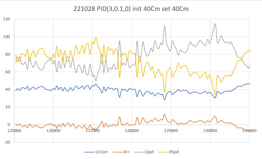
I was very encouraged by this run. The robot tracked very well for most of the run, deviating slightly at the very end. I’m particularly pleased by the 1.4sec period from about 129400 (129.4sec) to about 130800 (130.8sec); during this period the left & right wheel motor drive values were pretty constant, indicating that the PID was actively controlling motor speeds to obtain the desired the wall offset. I’m not sure what caused the deviation at the end, but it might have something to do with the ‘wall’ material (black art board with white paper taped to the bottom half) in that section. However, after replacing that section with white foam core, the turn-out behavior persisted, so it wasn’t the wall properties causing the problem.
After looking at the data and the video for a while, I concluded that the divergence at the end of the run was real. During the first part of the run, the robot was close enough to the setpoint so that no significant correction was required. However, as soon as the natural straight-line behavior diverged enough from the set point to cause the PID to produce a non-small output, the tracking performance was seriously degraded. In other words, the PID was making things worse, not better – rats.
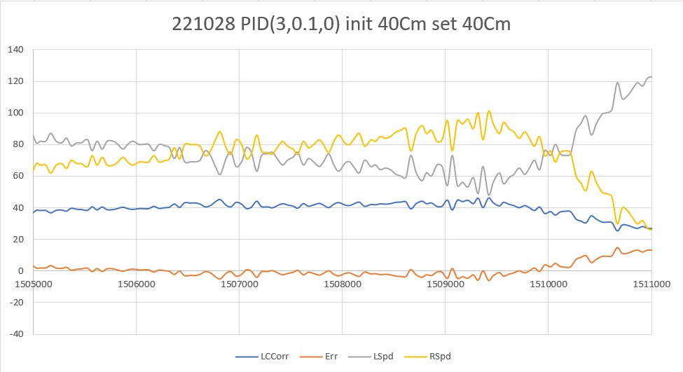
So, I tried another run, this time adding just a smidge of ‘D’, on the theory that this would still allow the PID to drive the robot back toward the setpoint, but not quite as wildly as before. With PID (3, 0.1, 0.1) I got the following plot:
As can be seen, things are quite a bit nicer, and the robot seemed to track fairly well for the entire 4m run.
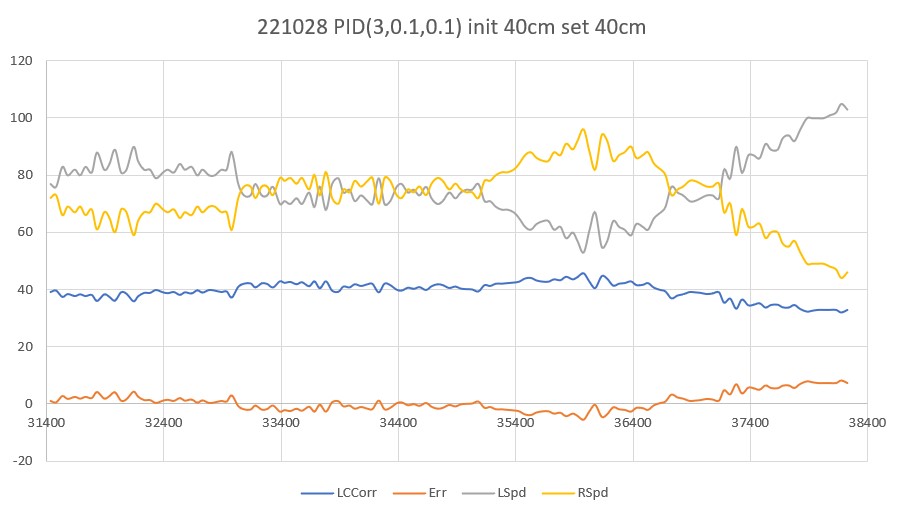
Tried another run this morning with PID(3,0,0.1), i.e. removing the ‘I’ factor entirely, but leaving the ‘D’ parameter at 0.1 as in my last run yesterday. As can be seen in the following plot and short video, the results were very encouraging.
Made another run with ‘D’ bumped to 0.5 – looks even better.
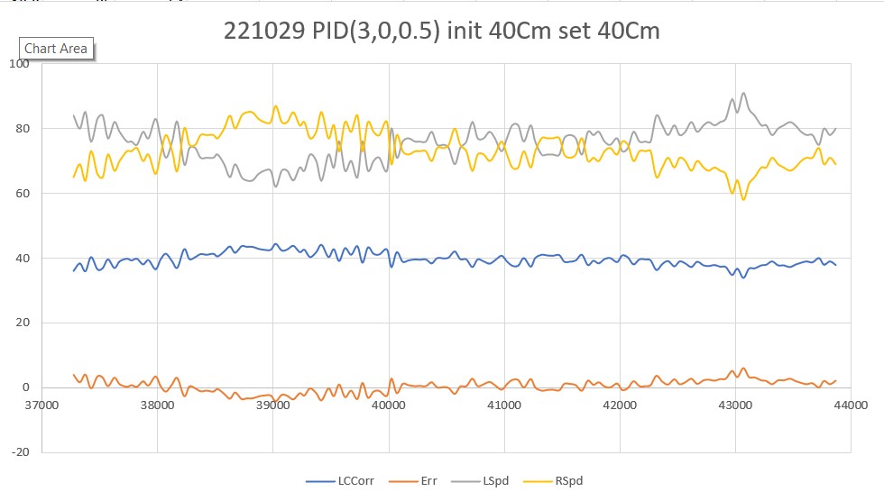
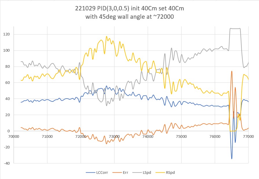
Next, I investigated Wall-E3’s ability to handle wall angle changes. As the following plot and video shows, it actually does quite well with PID(3,0,0.5)
30 October 2022 Update
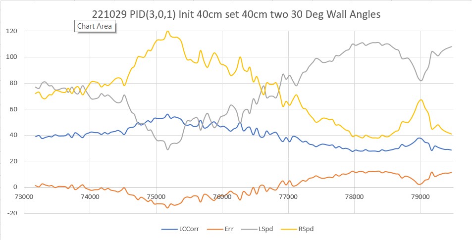
After a few more trials, I think I ended up with PID(3,0,1) as a reasonable compromise. With this setup, Wall-E3 can navigate both concave and convex wall angle changes, as shown in the following plot and short video.
As an aside, I also investigated several other PID triplets of the form (K*3,0,K*1) to see if other values of K besides 1 would produce the same behavior. At first I thought both K = 2 and K = 3 did well, but after a couple of trials I found myself back at K = 1. I’m not sure why there is anything magic about K = 1, but it’s hard to get around the fact that K = 2 and K = 3 did not work as well tracking my ‘sandbox’ walls.
At this point, I think it may be time to back-port the above results into my WallE3_AnomalyRecovery_V2.sln project, and then ultimately back into my main robot control project.
06 November 2022 Update:
Well, now I know why my past efforts at wall tracking didn’t rely exclusively on offset distance as measured by the 3 VL53L0X sensors on each side of the robot. The problem is that the reported distance is only accurate when the robot is parallel to the wall; any off-parallel orientation causes the reported distance to increase, even though the robot body is at the same distance. In the above work I thought I could beat this problem by compensating the distance measurement by the cosine of the off-parallel angle. This works (sort of) but causes the control loop to lag way behind what the robot is actually doing. Moreover, since there can be small variations in the distance reported by the VL53L0X array, the robot can be physically parallel to the wall while the sensors report an off-parallel orientation, or alternatively, the robot can be physically off-parallel (getting closer or farther away) to the wall, while the sensors report that it is parallel and consequently no correction is required. This is why, in previous versions, I tried to incorporate a absolute distance measurement along with orientation information into a single PID loop (didn’t work very well).
09 November 2022 Update:
After beating my head against the problem of tracking the nearby wall using a three-element array of VL53L0X distance sensors and a PID algorithm, I finally decided it just wasn’t wasn’t working well enough to rely on for generalized wall tracking. It does work, but has a pretty horrendous failure mode. If the robot ever gets past about 45 deg orientation w/r/t the near wall, the distance values from the VL53L0X sensor become invalid and the robot goes crazy.
So, I have been spending my night-time sleep preparation time (where I do some of my best thinking) trying to think of different ways of skinning this particular cat, as follows:
- The robot needs to be able to accurately track a given offset
- Must have enough agility to accommodate abrupt wall direction changes (90 deg changes are easy – but there are several 45 deg changes in our house)
- Must handle obstacles appropriately.
It’s that first item on the list that I can’t seem to handle with the typical PID algorithm. So, I started to think about alternative schemes, and the one I decided to experiment with was the idea of implementing a zig-zag tracking algorithm using my already-proven SpinTurn() function. SpinTurn() uses relative heading output from my MP6050 MPU to implement CW/CCW turns, and has proven to be quite reliable (after Homer Creutz and I beat MPU6050 FIFO management into submission).
I modified one of my Wall Track Tuning programs to implement the ‘zig-zag’ algorithm, and ran some tests in my office ‘sandbox’. As the following Excel plot and short video shows, it actually did quite well, considering it was the product of a semi-dream state thought process!
As can be seen from the above, the robot did a decent job of tracking the desired 40Cm offset (average distance for the run was 39.75Cm), especially for the first iteration. I should be able to tweak the algorithm to track the wall faster and with less of a ‘drunken sailor’ behavior.
Stay tuned,
Frank