Tag Archives: Charging Station

IR Modulation Processing Algorithm Development. Part XVI

Posted 22 July 2017

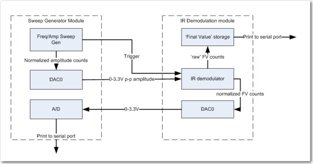
After getting the good news about the performance of my N-path filter for homing in on a 520Hz square-wave modulated IR beam, I still had two more significant tasks to accomplish; I still needed to extend the work to multiple (at least two) sensor channels for homing operation, and I needed to fully characterize the filter for frequency and amplitude response, and verify proper operation in the presence of ambient interference.

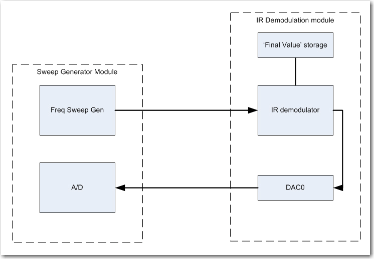
Second sensor channel:

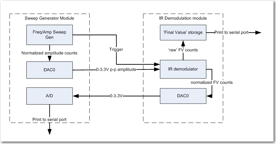
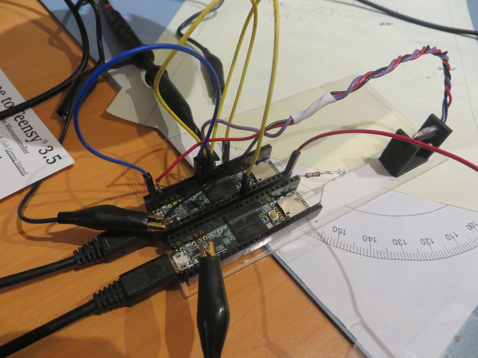
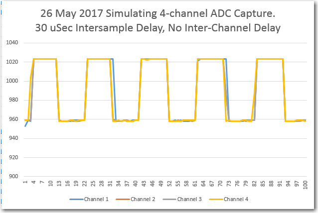
As it turned out, add a second channel to the demodulator/filter algorithm was a piece of cake, as I didn’t have to bother with ‘array-izing’ everything – I just added a second set of input & output pins for the second channel, and a second set of variables. Basically it involved doing a global replace of ‘variable_name’ with ‘variable_name1’, and then copying ‘variable_name1’ to ‘variable_name2′ wherever it occurred. As an added bonus, the Teensy 3.5 has two DAC channels, so I could route the final value for channel2 to the second DAC pin for ’round-trip’ measurements with the sweep generator – nice

Frequency/Amplitude/Interference characterization:

In wrapping my long and arduous journey toward a working 520Hz multi-sensor square-wave detector filter, I wanted to make a series of amplitude and frequency response plots for both banpass filter channels, and also figure out how to test for rejection of 60Hz & 60Hz harmonics.

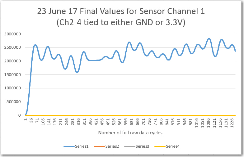
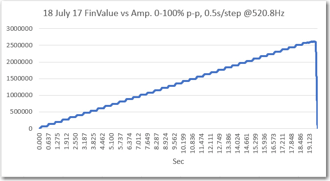
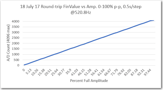
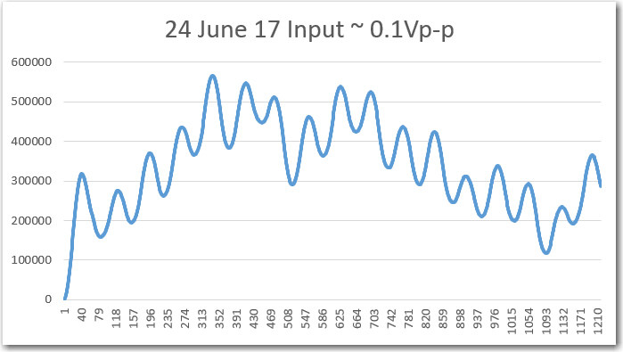
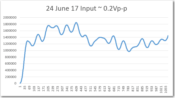
My initial amplitude sweep testing for channel 1 (original single channel) was very positive, as shown in the following plots:

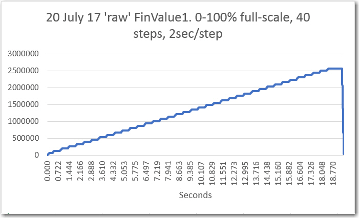
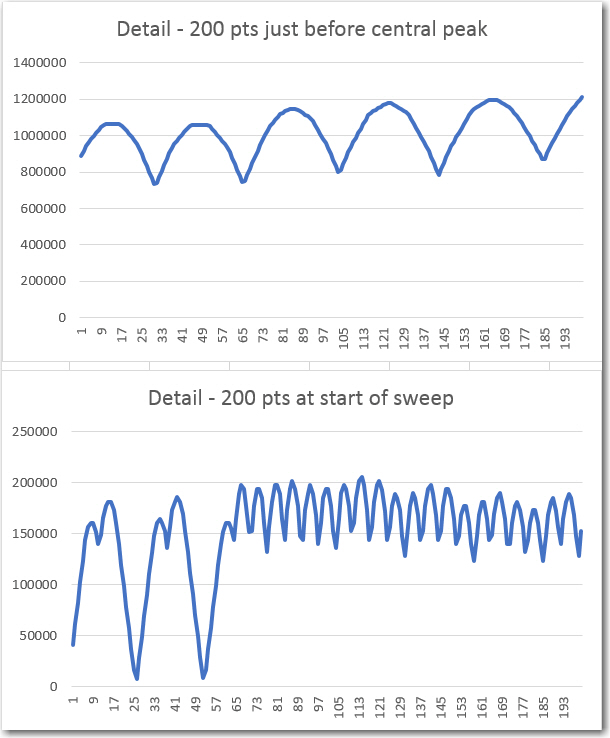
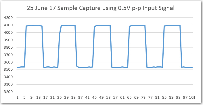
Channel 1 ‘raw’ amplitude response vs time

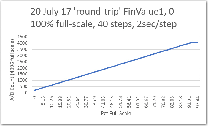
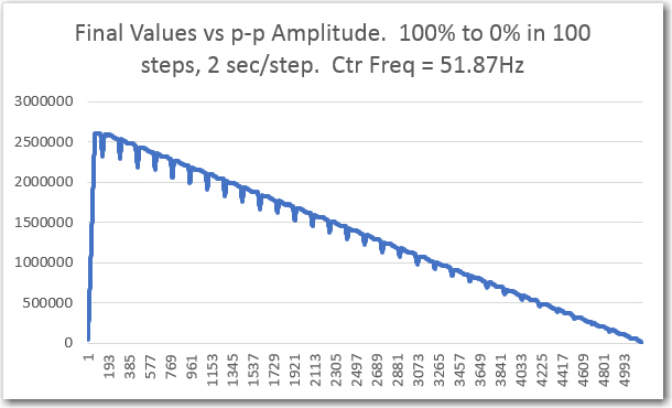
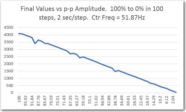
’round-trip (sweep gen -> IR Demod -> sweep gen) Channel 1 amplitude response vs input amplitude

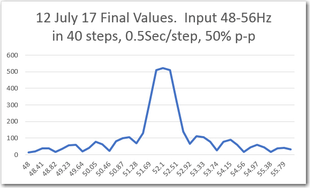
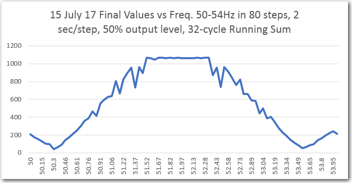
Channel1 Freq response

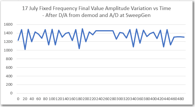
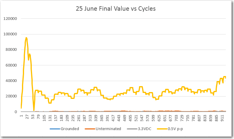
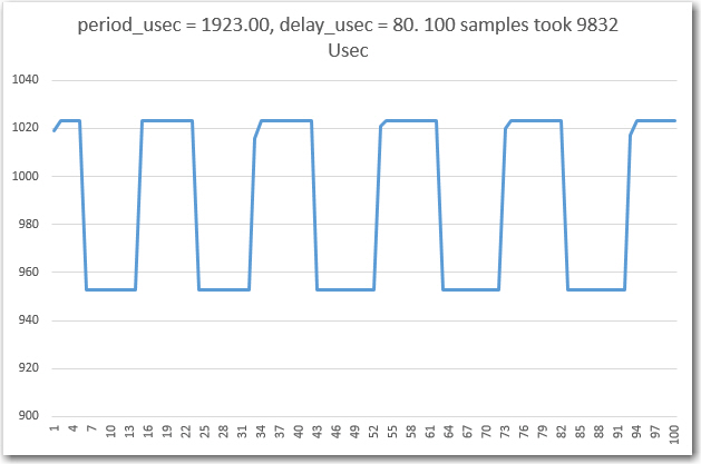
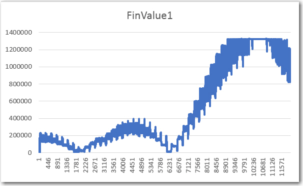
However, when I tried to run the frequency response curves, I ran into trouble (again!). As shown above, the plot was shifted significantly to the right, as if the demodulator’s frequency response had somehow shifted up in frequency. However, I knew from previous work that the demodulator center freq is 520.8Hz, so that couldn’t be the answer. The other possibility was that the sweep generator wasn’t producing the frequencies that I thought it was. Once I started thinking of this possibility, I remembered that a couple of days ago when I ran the very first fixed-amplitude response curves on the new-improved 520Hz demodulator, that I had been forced to tweak the sweep gen output freq to get the flat-line curve I was expecting. For convenience, I have repeated these plots below:

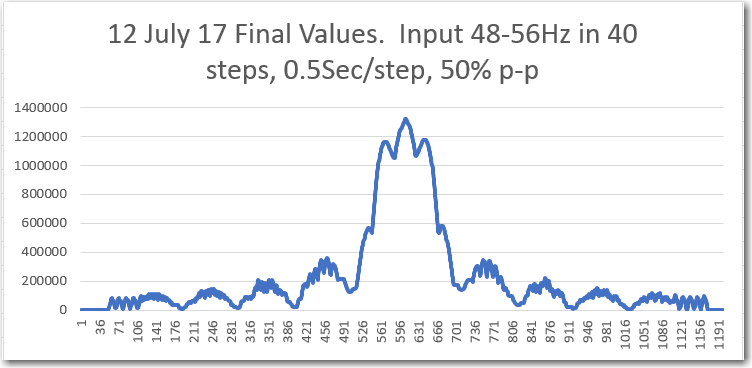
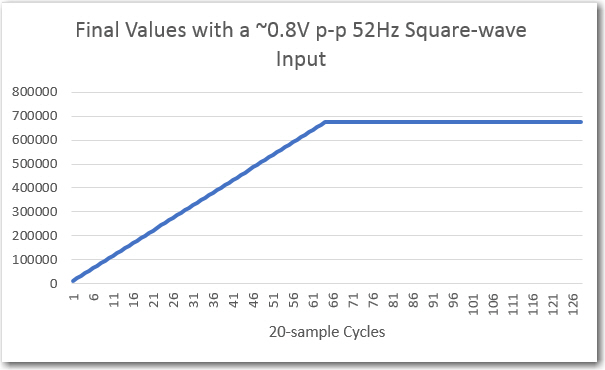
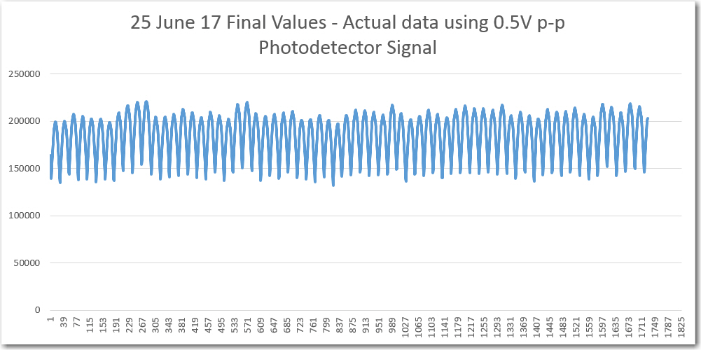
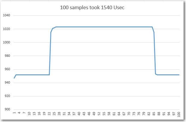
‘raw’ Final Values vs time, with fixed frequency, 50% p-p

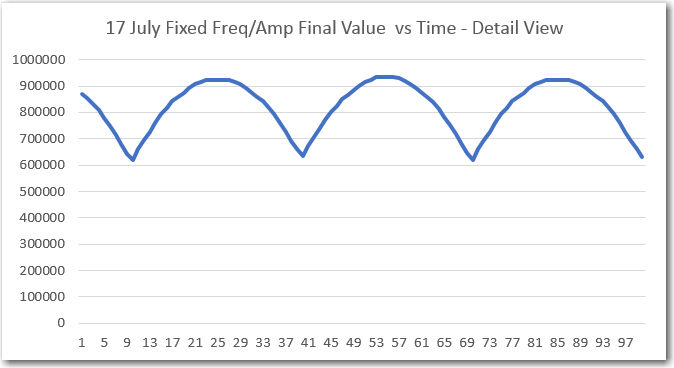
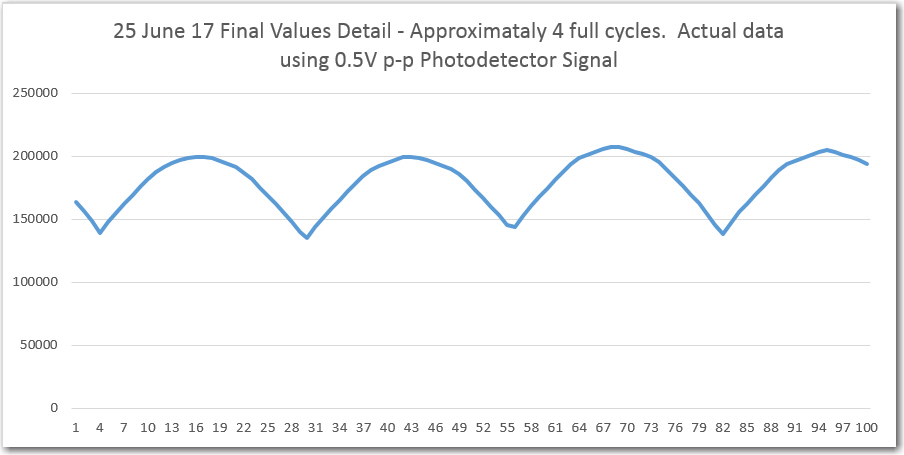
detail of ‘raw’ plot

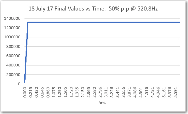
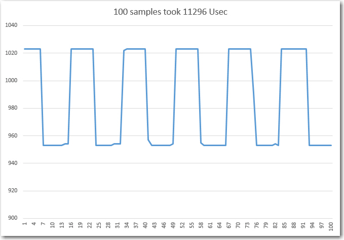
‘raw’ final values vs time after synching Tx & Rx frequencies

When I looked back into the sweep generator code, I found that its output frequency was set to 521.1Hz to produce a 520.8Hz output. At the time I didn’t think that was particularly egregious, but apparently is was a warning that I missed – oops!

So, now I embarked on yet another tangential project – this time to correct the frequency accuracy problems with the sweep generator module (which you might recall, was being used to test the IR demodulator, which in itself was a tangential project associated with the charging station project, which (you guessed it) was a tangential project in support of my Wall-E2 wall-following robot project. Talk about recursive! ;-).

Anyway, my first attempt at a swept-frequency generation algorithm wasn’t all that brilliant – just using ‘delayMicros()’ calls to create the square-wave as shown below:

{
float freqHz = FreqStart + i*freqstepHz;
//Serial.print("Step "); Serial.print(i + 1); Serial.print(" Freq = "); Serial.println(freqHz);

//compute required elapsed time for square wave transitions
sinceLastTransition = 0.5e6 / freqHz;

//output a square wave for the specified number of seconds
long startMsec = millis();
long stopMsec = millis();
while (stopMsec - startMsec < 1000* SecPerFreqStep)
{
	digitalWrite(SQWAVE_PIN, HIGH);
	analogWriteDAC0(DACoutHigh);
	digitalWrite(LED_PIN, HIGH);
	delayMicroseconds((int)sinceLastTransition);

	digitalWrite(SQWAVE_PIN, LOW);
	analogWriteDAC0(DACoutLow);
	digitalWrite(LED_PIN, LOW);
	delayMicroseconds((int)sinceLastTransition);

	stopMsec = millis(); //update the stop timer
}

{

float freqHz = FreqStart + i*freqstepHz;

//Serial.print("Step "); Serial.print(i + 1); Serial.print(" Freq = "); Serial.println(freqHz);

//compute required elapsed time for square wave transitions

sinceLastTransition = 0.5e6 / freqHz;

//output a square wave for the specified number of seconds

long startMsec = millis();

long stopMsec = millis();

while (stopMsec - startMsec < 1000* SecPerFreqStep)

{

digitalWrite(SQWAVE_PIN, HIGH);

analogWriteDAC0(DACoutHigh);

digitalWrite(LED_PIN, HIGH);

delayMicroseconds((int)sinceLastTransition);

digitalWrite(SQWAVE_PIN, LOW);

analogWriteDAC0(DACoutLow);

digitalWrite(LED_PIN, LOW);

delayMicroseconds((int)sinceLastTransition);

stopMsec = millis(); //update the stop timer

}

In retrospect it was clear that this was never going to produce frequency-accurate square-waves because of the additional time taken by the read/write statements. Without compensating for this additional delay, the output freq would always be below the nominal value, which is what I was experiencing.

Next, I modified the algorithm to use Teensy’s ‘elapsedMicros’ data type, as shown below, and ran a series of tests to determine its frequency accuracy.

	if (sinceLastTransition >= HalfCycleMicroSec)
	{
		if (transNum < SINCELAST_ARRAY_LENGTH)
		{
			aSinceLast[transNum] = sinceLastTransition; //stored for later analysis
		}
		else
		{
			Serial.println("Sweep terminated early - aSinceLast overflow!");
			DoSweepEnd(); //cleanup, offer to print, etc
		}

		sinceLastTransition -= HalfCycleMicroSec; //for most accurate timing
		transNum++;

		if (digitalRead(SQWAVE_PIN) == HIGH)
		{
			digitalWrite(SQWAVE_PIN, LOW);
			analogWriteDAC0(DACoutHigh * (1 - AmpPct / 100)); //level for this amp step
			digitalWrite(LED_PIN, LOW);
		}
		else
		{
			digitalWrite(SQWAVE_PIN, HIGH); //invert the output
			analogWriteDAC0(DACoutHigh); //level for this amp step
			digitalWrite(LED_PIN, HIGH);
		}

		//check for end of this step
		if (transNum >= numTransPerStep)
		{
			if (bIsFreqSweep) //change sqwv half-period
			{
				float curFreq = FreqStart + curStepNum*FreqStepVal;
				float nextFreq = curFreq + FreqStepVal;
				HalfCycleMicroSec = 5e5 / nextFreq;

				//print out Freq, Rx value
				Serial.print(curFreq);Serial.print("\t");
				Serial.print(HalfCycleMicroSec, 6);Serial.print("\t");
				Serial.print(analogRead(DEMOD_VALUE_READ_PIN));
				Serial.println();
			}
			else //change amplitude
			{
				AmpPct += AmpStepValPct;
				//stepVal = AmpPct;

				//print out amp val, Rx value
				Serial.print(AmpPct);Serial.print("\t");
				Serial.print(analogRead(DEMOD_VALUE_READ_PIN));
				Serial.println();
			}
			transNum = 0; //start a new count


			curStepNum++; //increment the step count
		}

		//check for end of sweep
		//Serial.print("curstep/numsteps"); Serial.print(curStepNum); Serial.print("/"); Serial.println(numSteps);
		if (curStepNum > numSteps)
		{
			Serial.println("Sweep ended successfully...");
			DoSweepEnd(); //cleanup, offer to print, etc
		}
	}
}//loop()

if (sinceLastTransition >= HalfCycleMicroSec)

{

if (transNum < SINCELAST_ARRAY_LENGTH)

{

aSinceLast[transNum] = sinceLastTransition; //stored for later analysis

}

else

{

Serial.println("Sweep terminated early - aSinceLast overflow!");

DoSweepEnd(); //cleanup, offer to print, etc

}

sinceLastTransition -= HalfCycleMicroSec; //for most accurate timing

transNum++;

if (digitalRead(SQWAVE_PIN) == HIGH)

{

digitalWrite(SQWAVE_PIN, LOW);

analogWriteDAC0(DACoutHigh * (1 - AmpPct / 100)); //level for this amp step

digitalWrite(LED_PIN, LOW);

}

else

{

digitalWrite(SQWAVE_PIN, HIGH); //invert the output

analogWriteDAC0(DACoutHigh); //level for this amp step

digitalWrite(LED_PIN, HIGH);

}

//check for end of this step

if (transNum >= numTransPerStep)

{

if (bIsFreqSweep) //change sqwv half-period

{

float curFreq = FreqStart + curStepNum*FreqStepVal;

float nextFreq = curFreq + FreqStepVal;

HalfCycleMicroSec = 5e5 / nextFreq;

//print out Freq, Rx value

Serial.print(curFreq);Serial.print("\t");

Serial.print(HalfCycleMicroSec, 6);Serial.print("\t");

Serial.print(analogRead(DEMOD_VALUE_READ_PIN));

Serial.println();

}

else //change amplitude

{

AmpPct += AmpStepValPct;

//stepVal = AmpPct;

//print out amp val, Rx value

Serial.print(AmpPct);Serial.print("\t");

Serial.print(analogRead(DEMOD_VALUE_READ_PIN));

Serial.println();

}

transNum = 0; //start a new count

curStepNum++; //increment the step count

}

//check for end of sweep

//Serial.print("curstep/numsteps"); Serial.print(curStepNum); Serial.print("/"); Serial.println(numSteps);

if (curStepNum > numSteps)

{

Serial.println("Sweep ended successfully...");

DoSweepEnd(); //cleanup, offer to print, etc

}

}//loop()

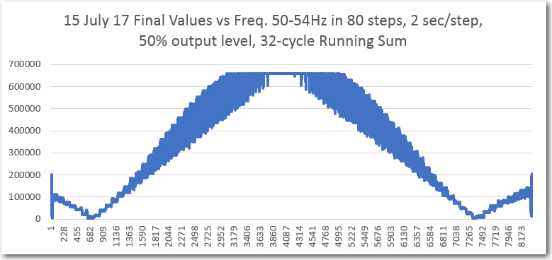
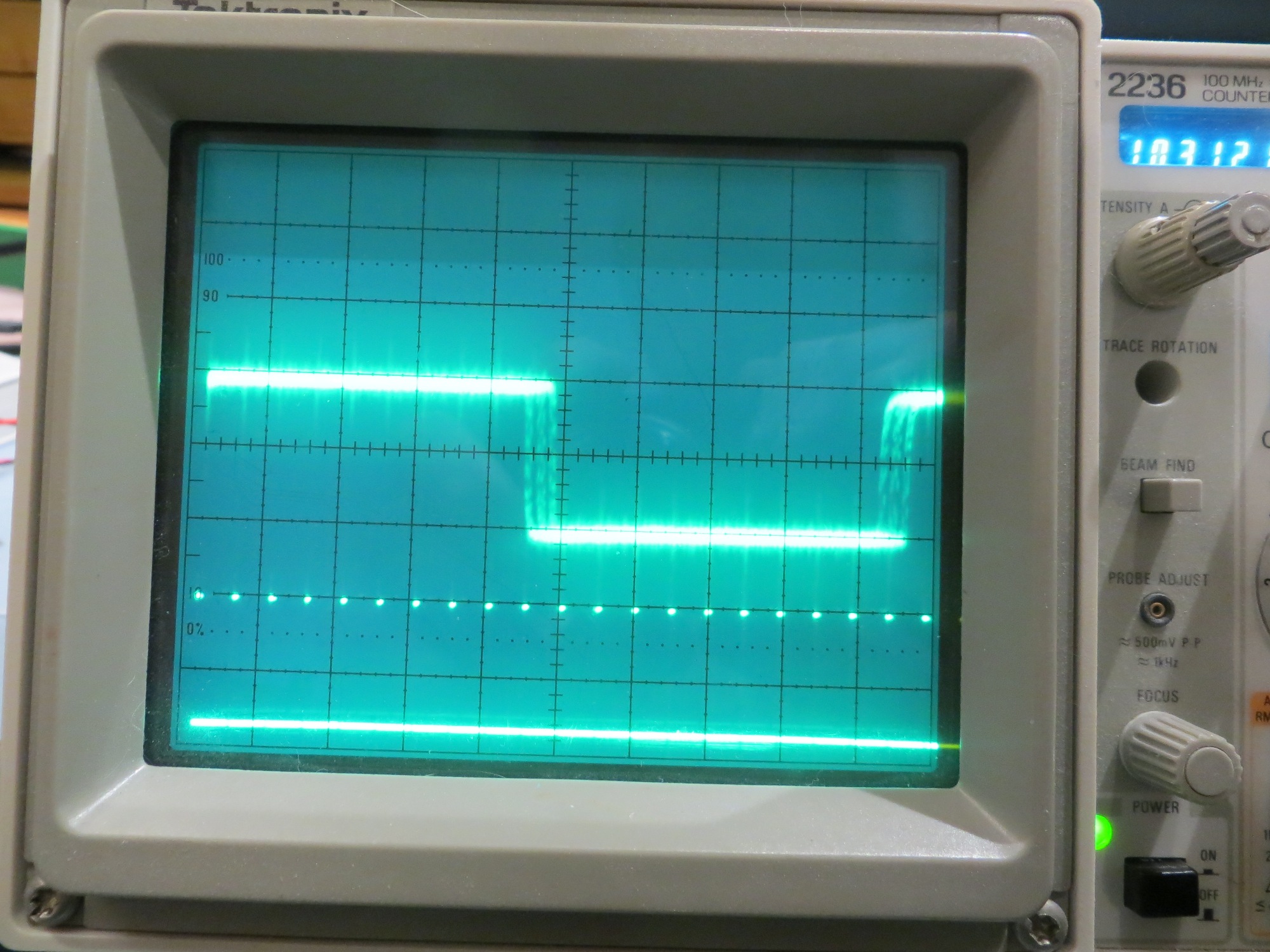
To test for frequency accuracy, I set the sweep generator to sweep from 501 to 531Hz with 50% output level and 5 sec/step. Then I measured the actual output frequency using my trusty Tektronix 2236 ‘scope with its built-in digital frequency readout. The results are shown below:

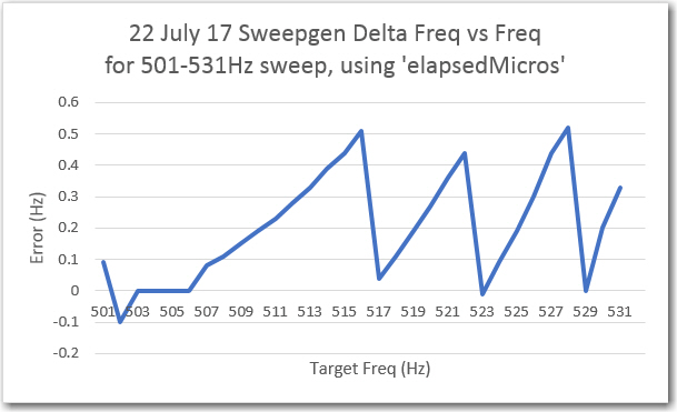
Frequency accuracy using the ‘elapsedMicros’ algorithm

This was OK, but not great, as it showed that the output frequency could be as much as 0.5Hz off from the expected value. After some web research (mostly on Paul Stoffregen’s wonderful Teensy forum), I decided to try the FrequencyTimer2 library described here. After implementing this in a separate test program, I ran the same frequency accuracy test as above, with the following results.

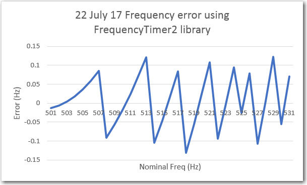
Frequency accuracy using the ‘FrequencyTimer2’ library

This was much better than the ‘elapsedMicros’ algorithm, but still not great; still greater than +/-0.1Hz deviation for some target frequencies.

Back to the web for more research, where I found the ‘IntervalTimer’ object described on this page. After modifying my test program to utilize this technique, I got the following results.

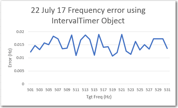
Frequency accuracy using the ‘IntervalTimer’ object

Wow! a lot better! Not only is the absolute error almost an order of magnitude less, the measured output frequency appears to be a constant 0.015Hz below (positive error) the target frequency. This leads me to believe that the frequency is probably right on the mark, and the error is in the measurement, not the timing. In any case, this technique is more than good enough for my puny little sweep generator! The complete test program used to generate these results is included below:

// Create an IntervalTimer object 
IntervalTimer myTimer;

const int ledPin = LED_BUILTIN;  // the pin with a LED
const int OUTPUT_PIN = 33;

void setup(void) 
{
	pinMode(ledPin, OUTPUT);
	pinMode(OUTPUT_PIN, OUTPUT);
	Serial.begin(115200);

	Serial.println("Freq\tTimerVal");
	for (size_t i = 501; i <= 531; i++)
	{
		float period = 1e6 / i;
		Serial.println(i);Serial.print("\t"); Serial.println(period);
		myTimer.begin(blinkLED, period/2);
		delay(5000);
		myTimer.end();
	}
	//myTimer.begin(blinkLED, 150000);  // blinkLED to run every 0.15 seconds
}

// The interrupt will blink the LED, and keep
// track of how many times it has blinked.
int ledState = LOW;
volatile unsigned long blinkCount = 0; // use volatile for shared variables

// functions called by IntervalTimer should be short, run as quickly as
// possible, and should avoid calling other functions if possible.
void blinkLED(void) 
{
	if (ledState == LOW) 
	{
		ledState = HIGH;
		//blinkCount = blinkCount + 1;  // increase when LED turns on
	}
	else {
		ledState = LOW;
	}
	digitalWrite(ledPin, ledState);
	digitalWrite(OUTPUT_PIN, ledState);
}

// The main program will print the blink count
// to the Arduino Serial Monitor
void loop(void) {
	//unsigned long blinkCopy;  // holds a copy of the blinkCount

	// to read a variable which the interrupt code writes, we
	// must temporarily disable interrupts, to be sure it will
	// not change while we are reading.  To minimize the time
	// with interrupts off, just quickly make a copy, and then
	// use the copy while allowing the interrupt to keep working.
	//noInterrupts();
	//blinkCopy = blinkCount;
	//interrupts();

	//Serial.print("blinkCount = ");
	//Serial.println(blinkCopy);
	//delay(100);
}

// Create an IntervalTimer object

IntervalTimer myTimer;

const int ledPin = LED_BUILTIN; // the pin with a LED

const int OUTPUT_PIN = 33;

void setup(void)

{

pinMode(ledPin, OUTPUT);

pinMode(OUTPUT_PIN, OUTPUT);

Serial.begin(115200);

Serial.println("Freq\tTimerVal");

for (size_t i = 501; i <= 531; i++)

{

float period = 1e6 / i;

Serial.println(i);Serial.print("\t"); Serial.println(period);

myTimer.begin(blinkLED, period/2);

delay(5000);

myTimer.end();

}

//myTimer.begin(blinkLED, 150000); // blinkLED to run every 0.15 seconds

}

// The interrupt will blink the LED, and keep

// track of how many times it has blinked.

int ledState = LOW;

volatile unsigned long blinkCount = 0; // use volatile for shared variables

// functions called by IntervalTimer should be short, run as quickly as

// possible, and should avoid calling other functions if possible.

void blinkLED(void)

{

if (ledState == LOW)

{

ledState = HIGH;

//blinkCount = blinkCount + 1; // increase when LED turns on

}

else {

ledState = LOW;

}

digitalWrite(ledPin, ledState);

digitalWrite(OUTPUT_PIN, ledState);

}

// The main program will print the blink count

// to the Arduino Serial Monitor

void loop(void) {

//unsigned long blinkCopy; // holds a copy of the blinkCount

// to read a variable which the interrupt code writes, we

// must temporarily disable interrupts, to be sure it will

// not change while we are reading. To minimize the time

// with interrupts off, just quickly make a copy, and then

// use the copy while allowing the interrupt to keep working.

//noInterrupts();

//blinkCopy = blinkCount;

//interrupts();

//Serial.print("blinkCount = ");

//Serial.println(blinkCopy);

//delay(100);

}

Before implementing the ‘IntervalTimer’ technique in my mainline sweep generator program, I re-ran the frequency sweep from 501 to 531Hz, with the following results.

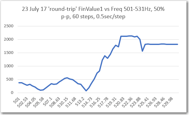
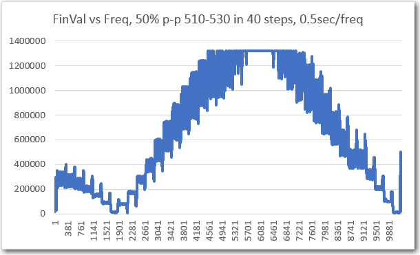
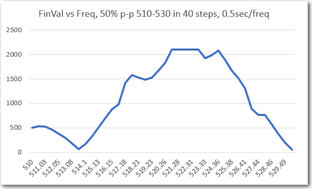
’round-trip’ freq sweep results before implementing the ‘IntervalTimer’ technique

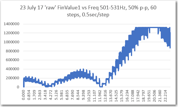
‘raw’ freq sweep results before implementing the ‘IntervalTimer’ technique

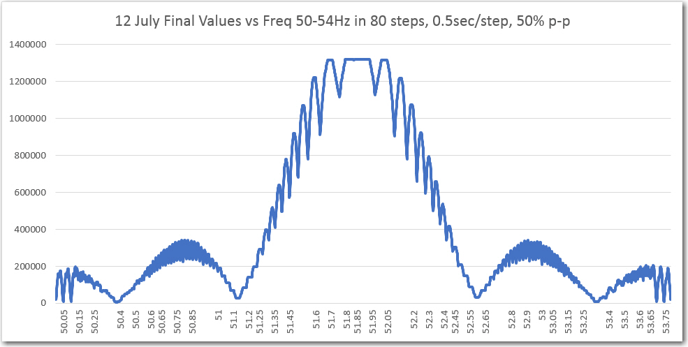
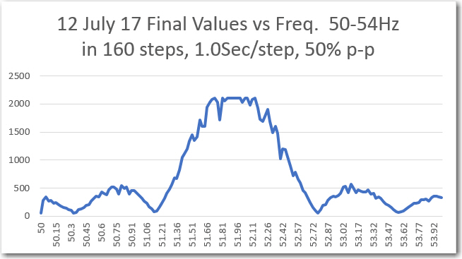
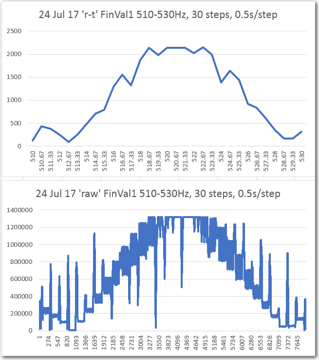
After implementing the new ‘IntervalTimer’ technique, I ran the sweeps again with nothing else changed, with the following results.

‘Round-trip’ and ‘raw’ FinalValue vs Frequency, with IntervalTimer technique

As can be seen from the above plots, they are nicely centered vs frequency, but the ‘raw’ plot has a lot of clearly ‘bad’ data – huge positive and negative excursions from the expected value.

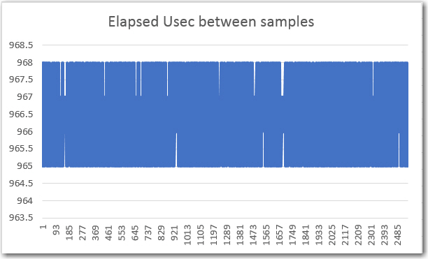
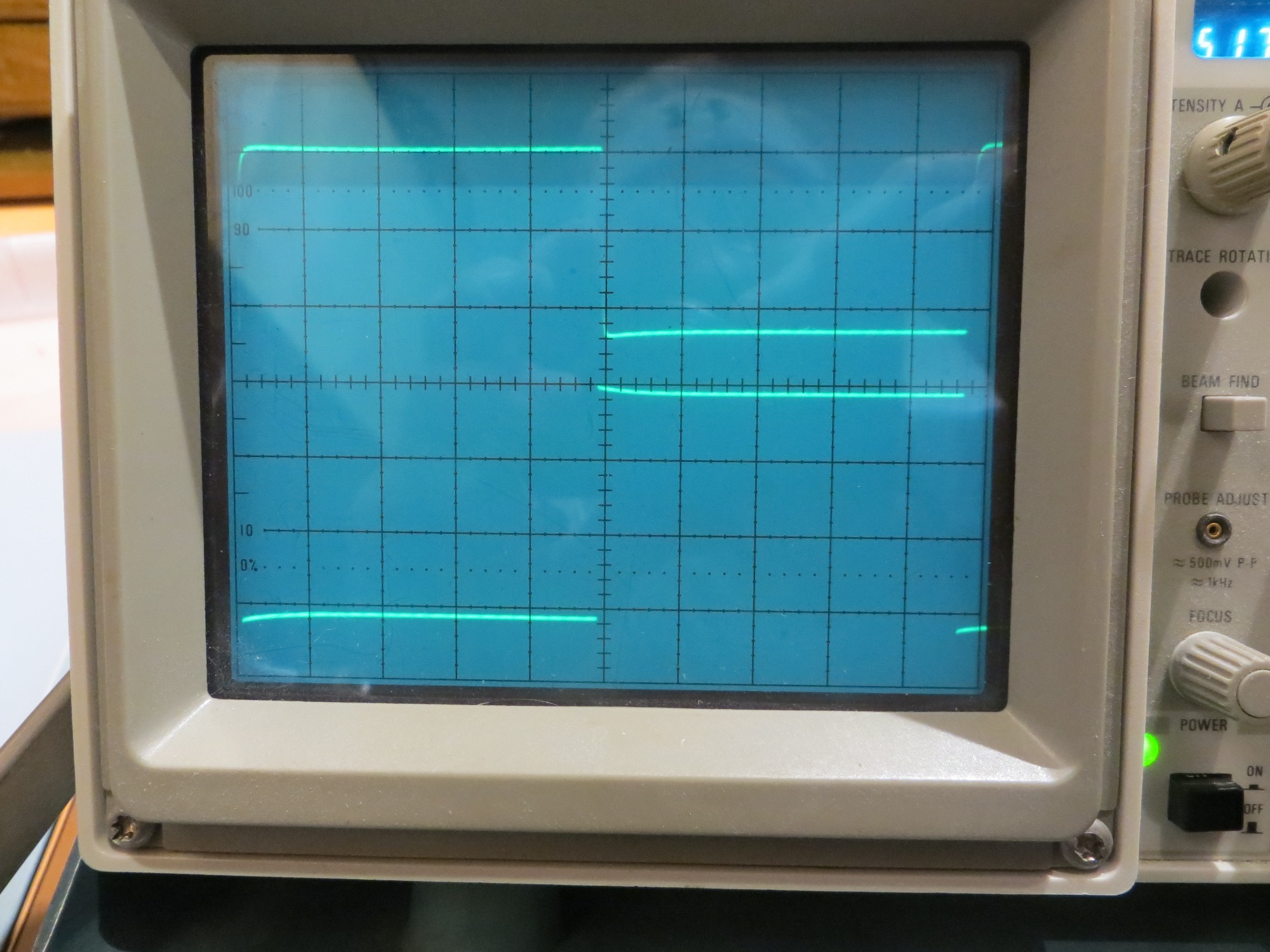
This situation led me down yet another rabbit-hole – what is causing these erroneous results? It appears that the bad data occurs at the beginning and the end of each 0.5 second frequency step – what could be causing that? After some thought, I decided to instrument the Interrupt Service Routine (ISR) that generates the square-wave transitions. As the following plot shows, there is a clear ‘glitch’ at the beginning of the first transition for each frequency step.

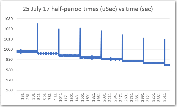
Square-wave transition times vs time using the IntervalTimer technique

Looking at the code that generates the sweep (shown below), it appears that the problem occurs because the IntervalTimer object must be destroyed (with ‘myTimer.end()’ and then re-created (with ‘myTimer.begin()’) with the new transition time. This inevitably causes the first transition of the next frequency step to be considerably off from nominal, and I don’t think there is anything I can do about it – bummer! 🙁

for (int i = 0; i <= FreqSteps; i++)
{
	float freqHz = FreqStart + i*freqstepHz;
	//Serial.print("Step "); Serial.print(i + 1); Serial.print(" Freq = "); Serial.println(freqHz);

	//compute required elapsed time for square wave transitions
	HalfCycleMicroSec = 0.5e6 / freqHz;
	myTimer.begin(SqwvGen, HalfCycleMicroSec);
	delay(SecPerFreqStep*1000);
	myTimer.end();
}

for (int i = 0; i <= FreqSteps; i++)

{

float freqHz = FreqStart + i*freqstepHz;

//Serial.print("Step "); Serial.print(i + 1); Serial.print(" Freq = "); Serial.println(freqHz);

//compute required elapsed time for square wave transitions

HalfCycleMicroSec = 0.5e6 / freqHz;

myTimer.begin(SqwvGen, HalfCycleMicroSec);

delay(SecPerFreqStep*1000);

myTimer.end();

}

So, it appears that my choices for accurate frequency generation are:

Use the ‘elapsedMicros()’ feature, with it’s inherent 0.5Hz max frequency error (due to rounding – this might be tweakable)
Use the ‘FrequencyTimer2’ library. This results in about 0.1Hz max error (again, possibly tweakable). Unfortunately, this technique requires that the output occur on a specific pin, which means I can’t output different levels without external hardware
Use the ‘IntervalTimer’ interrupt technique, which is very fast and very accurate. Unfortunately, as noted above, it also produces artifacts in the output spectra.

As I mentioned at the start of this post, this entire project is about three or four levels deep in the ‘tangential’ stack. The very last thing I wanted was yet another tangential project to learn the strengths/weaknesses of the various timing methods so I can implement the one with the best strength/weakness ratio, but yet here I am – arghhhh!

Stay tuned!

Frank

IR Modulation Processing Algorithm Development. Part XV

Leave a reply

Posted 18 July 2017,

In my last post on this (somewhat long-winded) subject, I described the implementation of a Teensy-based sweep generator utility for use in testing the band-pass filter (BPF) application, and showed some results from the 52Hz version of the BPF. As a result of this work, I believe I had validated both the test instrumentation and the 52Hz BPF implementation.

This post extends the previous work to the original goal for this project – the 520Hz BPF implementation. When I did the original work on the 520Hz version, it was clear there was something wrong, but not what. For reference, here are some representative plots from this 24 June 2017 post.

Computed final values vs complete input data cycles for sensor channel 1

There has been a lot of water over the dam between the 24 June post and now.

Replaced Trinket-based square-wave generator with Teensy 3.5 one for better frequency stability/accuracy
Replaced simple square-wave generator with frequency/amplitude sweep generator
Added ’round-trip’ measurement capability. Sweep generator -> BPF -> sweep generator so BPF response can be directly correlated to sweep generator output.
Revised BPF code to eliminate all but one sensor channel
Replaced all in-line printouts with writes to internal arrays, with post-run printout option.
Added micro-second accuracy time stamps to demodulator internal data capture
Temporarily reduced filter center freq from 520Hz to 52Hz to eliminate any possibility of timing problems due to Teensy 3.5 internal interrupts.

As the plots from the previous post showed, the 52Hz BPF implementation works as intended. So, it was time to try my hand (again!) with the 520Hz version. First, I did an elapsed time study, to make sure no sample periods were being missed. As the plot below shows, all the elapsed time values are reasonable, with only a few going to 101 Î¼Sec. I speculate that the 101 values may be due to execution of extra-long internal Teensy ISRs. The elapsed time plot conclusively demonstrates that something I did during the above list of changes eliminated the occasional (1 out of 68 or 69 cycles) missed sample that caused the previous ‘crappy’ results for the 520Hz version of the filter. My personal favorite for the culprit is one or more of the print statements I had in the original code for debugging.

Sample times vs time.

The next set of plots shows the results of an amplitude sweep, with the amplitude set to a fixed 50% p-p value

‘raw’ Final Values vs time, with fixed frequency, 50% p-p

’round-trip’ Final Values vs time, fixed freq, 50% p-p

detail of ‘raw’ pot

The above plots weren’t quite what I expected; both the ‘raw’ and ’round-trip’ final values were lower than expected, and the ‘raw’ plot had a lot more ripple than I wanted to see. This all led me to believe that the test frequency was not centered in the BPF passband. I had not actually double-checked this, so I went back a few steps and made sure the fixed amplitude sweep frequency was indeed synched with the demodulator sampling frequency. After that, the plots got a lot cleaner, as shown below.

‘raw’ final values vs time after synching Tx & Rx frequencies

In the above plot, the ‘raw’ final value is pretty steady around the value 1,320,000, which agrees well with a 50% p-p Tx level.

Next, I ran frequency sweeps, as shown in the following plots

‘raw’ Final Values vs frequency, with amplitude @ 50% p-p

’round-trip’ Final Values vs frequency, with amplitude @ 50% p-p

For reference, the same two plots for the 52Hz implementation are shown below

Captured ‘raw’ final value from IR demodulator. Frequency values added later

Frequency sweep results from sweep generator printout (D/A from IR demod, then A/D in sweep gen)

Next, I ran an amplitude sweep from 0% to 100% p-p input, as shown in the following plots

‘raw’ Final Values vs amplitude, with frequency @ 520.8Hz

’round-trip’ Final Values vs amplitude, with frequency @ 520.8Hz

So, it appears to me that the 520Hz BPF is working just as well as the 52Hz one, and it’s time to move on to multi-sensor operation.

I have placed the code for the now working 52/520Hz single-channel N-path BPF on GitHub at https://github.com/paynterf/SqWaveIQDemodV2.git. There are three branches available on GitHub, as follows:

Master – this is the original ‘root’ for the IQ Demodulator (BPF) project
SingleChannel – this is the final code for the single channel version, working at 52 & 520Hz
TwoChannel – this is my new branch to host the in-progress dual-channel BPF.

Stay tuned!

Frank

IR Modulation Processing Algorithm Development. Part XIV

1 Reply

Posted 07 July 2017

In my last post on this subject, I described a working 52Hz implementation of John Jenkins’ ‘degenerate N-Path Band-pass filter (BPF). This filter is intended to allow Wall-E2 (my wall-following robot) to discriminate between the IR homing beam from a charging station and other ambient IR interferers. This post describes the implementation of a basic swept-frequency square-wave function generator for use in testing BPF performance.

Now that I have a working (I think) version of the BPF algorithm, I want to implement and test a frequency and amplitude sweeping module so I can use it to test not only the working 52Hz BPF implementation, but the (so far not working) 520Hz implementation when we finally get the bugs worked out of it. My idea is that doing this now will have two (maybe three) significant benefits

Allows me to fully characterize the existing 52Hz BPF implementation
Gives me baseline performance characteristics for comparison against 520Hz results
(freebie) – More fun with Teensy!

I’m already using a second Teensy 3.5 as the 52Hz square wave transmitter in my test setup, so all I need to do is to modify the existing program to sweep the desired frequencies and amplitudes. I think I’ll do this as a command-line parameter-entry program, with user-entry parameters for start, stop, and step frequencies (Hz) and fixed amplitude (% full-scale) for the frequency sweep module, and start, stop, and step amplitudes (% full-scale) and a set center freq for the amplitude sweep module.

12-15 July 2017 Update:

Well, I finally got the sweep generator going, at least the frequency sweep part, and managed to get some good data out of the 52Hz square wave demodulator. What I was striving for was something akin to the normal hardware setup where a frequency-sensitive ‘device under test’ (DUT) is driven from a frequency sweep generator, and a data logger of some sort records the result, something like the following block diagram. Back in the day, the ‘datalogger’ was quite often an engineer recording results on a piece of graph paper – how quaint! 😉

Typical swept frequency test setup

In this project, the DUT is the Teensy 3.5 hosting the IR demodulator code, and the frequency sweep generator is another Teensy 3.5 hosting the code to generate a swept-frequency square wave signal.

But, what to do about the datalogger? I could record data from inside the demodulator program, but we’re talking a lot of data; even at 52Hz that’s 52 4-byte values per second, and a sweep test might take as long as 3 minutes –> 36000 bytes. Fortunately, the Teensy 3.x sports 192KB of RAM, so a 36KB chunk barely scratches the paint – yay!! Another problem with logging internal to the demod module is how to correlate the captured data with the driving frequency; they are obviously correlated, but it’s not a slam-dunk to unequivocally assign particular frequencies to a particular stored data value.

So, I decided on a two-pronged approach; I will indeed save the data internally to RAM for later printout, but will also output an appropriately scaled version of the ‘final value’ calculation to one of the two DAC ports available on the Teensy 3.5 SBC. I plan to run this signal back to the sweep generator module so I can correlate ‘final value’ values with test frequencies, as shown in the following amended block diagram.

Modified sweep test block diagram

This setup works, and now I can get frequency-correlated ‘final value’ data from the sweep generator A/D. However, since the demodulator module ‘free-runs’ with respect to the sweep generator, the final value storage array can fill up before the frequency sweep finishes (or even before it starts!), so something is needed to synch the two modules. As the following block diagram shows, this is accomplished by providing a digital trigger from the sweep generator to start the demodulator. Also added in this final setup is the ability to set the square wave amplitude, for later amplitude sweep tests (set to 50% amplitude for the swept-frequency tests)

Final sweep setup. Note DAC block for square wave amplitude adjustment and trigger signal for synchronization

With the above setup I ran a number of frequency sweeps, as shown in the plots below. I started out with a sweep from 48 to 56Hz (+/- 4Hz from center freq), but quickly narrowed it down to +/- 2Hz. As my friend and mentor John Jenkins pointed out in his gentle, diplomatic way (something like “What were you thinking!“), the BPF bandwith is less than 1Hz, so a +/- 4Hz sweep range will just record a lot of nothing – oops!

Frequency sweep results from sweep generator printout (D/A from IR demod, then A/D in sweep gen)

Captured ‘raw’ final value from IR demodulator. Frequency values added later

Even though the above sweeps were way too wide, it is clear that the demodulator algorithm is working (at least in the 52Hz implementation).

Frequency sweep results from sweep generator printout (D/A from IR demod, then A/D in sweep gen)

Captured ‘raw’ final value from IR demodulator. Frequency values added later

In the above plots, the sweep was reduced to +/- 2Hz, and the number of steps increased to 80. The result is a much more detailed look at the BPF response. As expected the general shape of the ’round-trip’ (individual ‘final value’ numbers sent from the demodulator to the sweep generator via the DAC-A/D channel and then printed) plot and the ‘raw final value’ plot match, but I didn’t expect either the flat-top region at the center of both plots or the fine ripple shown in the ‘raw’ plot. I made a number of additional sweeps with up to 160 steps at 2 sec/step, but neither the flat-top region nor the fine ripple features changed – they are apparently real features of the BPF response.

I think I finally figured out that the flat-top region was due to the fact that there is a narrow range of frequencies for which the filter response is maximum and identical. In this very narrow region, the digital sample points are ‘perfectly’ aligned with the incoming square wave, so that the final value is the maximum possible value for the input p-p amplitude.

As for the fine ripple features, I think these are due to the beat frequency between the incoming signal and the sample period. If this is the case, I would expect the ripple features to be more closely spaced far away from the center frequency, and less closely spaced toward the center. This certainly seems to be the case in the above plot, but even more evident in the detail plots below, (points extracted from the main plot above)

far and near center BPF response detail

Next, I performed an amplitude sweep from 100% to 0% p-p amplitude, with the center frequency set to 51.87Hz (this value was empirically determined earlier), with the following results

‘Raw’ final values from amplitude sweep.

final values captured by sweep generator

As the above plots show, the filter response is very linear with respect to p-p amplitude variations. The maximum value shown in the ‘raw’ plot above is a little above 2.5 x 10⁶. The actual maximum value from the data is 2,606,752, which matches well with the theoretical maximum value of 4096*10*64 = 2,621,440.

Lastly, I performed another frequency sweep, but this time with a running-sum length of 32 cycles vs 64, to see how much the band-pass width was affected by halving the number of cycles in the running-sum circular buffer. Comparing the 32-cycle and 64-cycle plots as shown below, the ‘flat-top bandwidth is considerably wider than the original 64-cycle sweep results – about 1.8Hz edge-to-edge for 32 and about 0.4 for the original 64 version. Maybe as much as 4x bandwidth increase.

Frequency sweep results from sweep generator printout (D/A from IR demod, then A/D in sweep gen)

Frequency sweep results from sweep generator printout (D/A from IR demod, then A/D in sweep gen)

Captured ‘raw’ final value from IR demodulator.

Summary and Conclusions:

This post described my efforts to characterize the frequency and amplitude responses for the 52Hz implementation of the ‘degenerate N-path band-pass filter’ described to me by friend and mentor John Jenkins some time ago.

The original plan was to use this filter technique at 520Hz to enable my Wall-E2 wall-following robot to home to a charging station using a square-wave modulated IR signal to suppress ambient IR interference. Unfortunately, I could not get the 520Hz implementation to work properly, probably due to some unknown timing issues associated with the Teensy 3.x architecture. So, I decided to run the filter at 1/10th speed (52Hz) instead, thereby eliminating any timing issues, and allowing me to establish a baseline for subsequent higher-speed testing.

As the data above shows, the effort to implement the N-path BPF at 52Hz was completely successful. Both the frequency and amplitude responses were characterized. In addition:

I gained a lot more experience with the Teensy 3.x line of SBCs. They are less than half the size of an Arduino Uno, have over 10x more RAM, 50x faster, come with on-board SD (3.5 & 3.6) cost about the same, and have about the same power requirements – such a deal!
Implemented a Teensy 3.5 frequency/amplitude sweep square wave generator, and verified proper operation by using it to characterize the 52Hz BPF implementation.
Implemented a Teensy 3.5 fixed-frequency square wave generator, and verified proper operation by using it to find the correct transmit frequency for the 52Hz BPF implementation
Validated the efficacy of my little two-Teensy test bed.

The above tools can now be used with high confidence to investigate (and hopefully eliminate) the problems with running the BPF at 520Hz.

Stay tuned!

Frank

IR Modulation Processing Algorithm Development. Part XIII

1 Reply

Posted 03 July 2017

With this post, I’m nearing a new Personal Record for a subject series (the ‘Charging Station Design’ series went to 14), with no end in sight. The last missive from my friend and mentor John Jenkins (I’m reconsidering the ‘friend’ part, as ASFAICT, he intends to drive me into an early grave over this project!) was ‘Still not there – the ‘Final Value’ output from the filter is still wrong! :-(.

Be that as it may, it is my lot, challenge, ‘opportunity to excel’ or whatever, to continue working on this thing until I kill it – or it kills me (indeterminate as to which at the moment) 😉

So, after eliminating most/all of the print statements, John is still convinced that the Teensy is missing samples on a regular basis, and this is screwing up the rest of the algorithm. I’m just as convinced that the Teensy is way too fast to miss any samples, and that any problems must be later in the algorithm.

However, there may be a way to settle which is which, without the use of magic or a crystal ball. The Teensy 3.5/3.6 SBC’s come with a built-in micro-SD card capability, which I think can be used to log the output of each stage in a way that doesn’t (I hope) impact sample timing.

The first step in my new master plan is to make sure I can actually write to and read from an SD card on my demod Teensy (actually my first step was to go by MicroCenter and get a micro-SD card, as all mine seem to have disappeared!). I found and loaded PaulStoffregen Paul Stoffregen’s nice little SD test sketch from his GitHub site, and ran it on my Teensy 3.5. After changing the ‘chipSelect’ constant from the default 4 to ‘BUILTIN_SDCARD’, it ran successfully, and I was even able to open the ‘Test.txt’ on my PC – Yay!

The next step is to modify my IR demod program to send logging data to the SD card instead of the serial port, and to monitor my timing pulse output to make sure the SD card writes don’t interfere (can’t imagine they would, but I have a very limited imagination!).

After timing a loop that wrote 1000 short lines to the SD card, I reluctantly came to the conclusion that the stock SD card library may not be fast enough to ensure that logging output isn’t affecting the results of the algorithm. There is a faster library (SdFat), and some other speedup techniques, but rather than going down yet another rabbit-hole, I decided it was time to try a different idea.

The original plan for the IR demod idea was to use a ~520Hz square-wave modulation frequency. This is high enough to be well away from 60Hz line freq, and not aligned with higher line harmonics, but it may be just high enough to be causing the problems we are seeing. Since the algorithm actually doesn’t care what the frequency is, I decided that I can put the timing issue to bed by simply reducing the modulation frequency by a factor of 10, to something like 52Hz. Sample spacing at this frequency (assuming 20 samples/cycle) is 1000Î¼S, which should provide more than enough room for computations (and hopefully some printouts).

To start this process, I modified both the transmit and receive Teensy 3.5 programs for the new, lower freq, and then tweaked the transmit frequency to synch with the receiver timing. As the following short video shows, a transmit frequency of 51.87Hz and a receive frequency of 51.815Hz synched up fairly well.

The demodulator timing pulse train (the rising edge is at the start of the sampling/computation block,and the trailing edge is at the end) is shown in the following scope photos.

Bottom trace is sampler pulse train, top trace is square wave at ~52Hz. Time scale is 1ms/cm

Photo showing just one sampling period. Time scale is 0.1ms/cm

Expanded view of one sampling/computation period. Time scale is 5 microsec/cm

From the above photos, it is clear that the entire sampling/computation block takes less than 10Î¼S, leaving about 990Î¼S free before the next sample occurs.

Yesterday, ‘talking’ about this problem (‘talking’ with John can be a rather terrifying experience – sort of like ‘talking’ with Zeus – you wonder when the thunderbolt will arrive and whether or not he’s going to miss) with John, I opined that if his theory of missing samples is correct, a list of accurate sample timestamps should show some gaps; a linearly increasing timestamp value would refute the claim, and a plot with vertical jumps would validate it.

Then last night, as I was drifting off to sleep, I realized I didn’t have to actually create the necessary timestamps, as I already had them in the code. The elapsedMicros variable type such as ‘sinceLastSample’ gets incremented by the system each time through loop(), and only gets modified from inside the sampling/computation loop. If all samples are taken on time, this variable should be a constant when measured inside the sample/computation block just before it gets reset. The relevant code snippet is shown below

	//this runs every 95.7uSec
	if (sinceLastSample > USEC_PER_SAMPLE)
	{
		/*RECORD sinceLastSample HERE!*/

		//sinceLastSample = 0;
		sinceLastSample -= USEC_PER_SAMPLE;

//this runs every 95.7uSec

if (sinceLastSample > USEC_PER_SAMPLE)

{

/*RECORD sinceLastSample HERE!*/

//sinceLastSample = 0;

sinceLastSample -= USEC_PER_SAMPLE;

At the point shown by “/*RECORD sinceLastSample HERE!*/” in the above snippet, the ‘sinceLastSample’ variable should be USEC_PER_SAMPLE +/- 1Î¼S. A dropped sample event should cause the value of this variable to change to N*USEC_PER_SAMPLE, where N is the number of consecutive dropped samples.

So, all I have to do is write the ‘sinceLastSample’ value to an array for a few seconds, and then write it back out again after stopping the program. An Excel plot of the values should tell the tale, one way or the other

05 July 2017

Here are some preliminary results from the 52Hz implementation

A 2560-point (128 cycles) array containing ‘sinceLastSample’ values.

129-point array containing ‘Final Value’ values

Note that the ‘sinceLastSample’ value varies -0/+3 Î¼S from ideal (the actual value is something like 964.32 Î¼S), and there are clearly no dropped samples.

The ‘Final Value’ curve looks rather linear up to something like 680,000, which I suspect John is going to confirm is the correct value for a 0.8V p-p squarewave input at the center freq of the filter passband.

So, assuming John does indeed confirm the final value numbers are correct, pretty much validates the algorithm (unchanged from the 520Hz version), and lends credence to his idea that samples are getting dropped in the higher frequency implementation.

More to come,

Frank

IR Modulation Processing Algorithm Development. Part X

1 Reply

Posted 24 June 2017

Well, I may have spoken too soon about the perfection of my implementation of John’s ‘N-path’ band-pass filter (BPF) intended to make Wall-E2 impervious to IR interference. After my last post on this subject, I re-ran some of the ‘Final Value’ plots for different received IR modulation amplitudes and the results were, to put it bluntly, crap 🙁 . Shown below is my original plot from yesterday, followed by the same plot for different input amplitudes

Computed final values vs complete input data cycles for sensor channel 1 (This is the original from yesterday)

So, clearly something is ‘fishy in Denmark’ here, when the ‘no-signal’ case with only high-frequency noise causes the output to increase without limit, and the ‘input grounded’ case is decidedly non-zero (although the values are much lower than in the ‘signal present’ cases).

Time to go back through the entire algorithm (again!) looking for the problem(s).

25 June 2017

My original implementation of the algorithm was set up to handle four sensor input channels, so each step of the process required an iteration step to go through all four, something like the code snippet below:

//Step1: Collect a 1/4 cycle group of samples for each channel and sum them into a single value
// this section executes each USEC_PER_SAMPLE period
for (int i = 0; i < NUMSENSORS; i++)
{
	//07/20/17 rev to capture raw data for later readout
	int samp = adc->analogRead(aSensorPins[i]);
	aSampleSum[i] += samp;
}
SampleSumCount++; //goes from 0 to SAMPLES_PER_GROUP-1

//Step1: Collect a 1/4 cycle group of samples for each channel and sum them into a single value

// this section executes each USEC_PER_SAMPLE period

for (int i = 0; i < NUMSENSORS; i++)

{

//07/20/17 rev to capture raw data for later readout

int samp = adc->analogRead(aSensorPins[i]);

aSampleSum[i] += samp;

}

SampleSumCount++; //goes from 0 to SAMPLES_PER_GROUP-1

In order to simplify the debug problem, I decided to eliminate all these iteration steps and just focus on one channel. To do this I ‘branched’ my project into a ‘SingleChannel’ branch using GIT and TortoiseGit’s wonderful GIT user interface (thanks TortoiseGit!). This allows me to muck about in a new sandbox without completely erasing my previous work – yay!

Anyway, I eliminated all the 4-sensor iteration steps, and went back through each step to make sure each was operating properly. When I was ‘finished’ (I never really finish with any program – I just tolerate whatever level of bugs or imperfections it has for some time). After this, I ran some tests for proper operation using just one channel. For these tests, the Teensy ADC channel being used was a) grounded, b) connected to 3.3VDC, c) unterminated. For each condition I captured the ‘Final Value’ output from the algorithm and plotted it in Excel, as shown below.

Single channel testing with grounded, unterminated, and +3.3VDC input

As can be seen from the above plot, things seem to be working now, at least for a single channel. The ‘grounded’ and ‘3.3VDC’ cases are very nearly zero for all time, as expected, and the ‘unterminated’ case is also very low.

Next, I added a 0.5V p-p signal at ~520Hz to the sensor input, and re-ran the program. After capturing the ‘Final Value’ data as before, I added it to the above plot, as shown below

Final Value vs Cycles for 0.5V p-p input

As can be seen in the above plot, the ‘Final Value looks much more reasonable than before. When plotted on the same scale as the ‘grounded’, ‘unterminated’, and ‘+3.3VDC’ conditions, it is clear that the 0.5V p-p case is a real signal.

Then I ran a much longer term (11,820 cycles, or about 22-23 sec) test with 0.5V p-p input, with the following results.

As can be seen from the above plot, the final value is a lot more ‘spiky’ than I expected. The average value appears to be around 30,000, but the peaks are more like 60,000, an approximately 3:1 ratio. With this sort of variation, I doubt that a simple thresholding operation for initial IR beam detection would have much chance of success. Hopefully, these ‘spikes’ are an artifact of one or more remaining bugs in the algorithm, and they will go away once I find & fix them 😉

Update: Noticed that there was a lot of time jitter on the received IR waveform – wonder if that is the cause of the spikes?

sensor waveform jitter. Note that this display is separately (Vert Mode) triggered.

Following up on this thread, I also looked at the IR LED (transmit) and photodetector (receive) waveforms together, and noted that there is quite a bit of time jitter on the Tx waveform as well, and this is received faithfully by the IR photodetector, as shown in the following short video clip

So, based on the above observations, I decided to replace the Trinket transmit waveform generator with another Teensy 3.5 to see if I could improve the stability of the transmit signal. Since I never order just one of anything, I happened to have another Teensy 3.5 hanging around, and I soon had it up and running in the setup, as shown below

Replaced Trinket transmitter with Teensy 3.5

Transmit and receive waveforms

As the above short video and photos show, the Teensy implementation of the transmit waveform is much more stable than the Trinket version. Hopefully this will result in better demodulation performance.

The next step was to acquire some real data using a 0.5V p-p input signal through the IR beam path. I took this in stages, first verifying that the raw samples were an accurate copy of the input signal, and then proceeding on to the group-sum, cycle-sum, and final value stages of the algorithm.

Sample capture using an input of 0.5V p-p through the IR path

GroupSum I/Q plots using 0.5V p-p Input Signal

I then used Excel to compute the cycle sums associated with each group of 4 group sums

Calculated Cycle Sums for a 0.5V p-p Input Signal

And then I used Excel again to calculate the ‘Final Value’ from the previously calculated cycle sum data

Calculated final value

Keep in mind that all the above plots are generated starting with real IR photodector data, and not that large of an input at that (0.5V p-p out of a possible 3.3V p-p).

The next step was the real ‘proof of the pudding’. I ran the algorithm again, but this time I simply printed out final values – no intermediate stages, and got the following plots

Final Value vs time, for 0.5V p-p Input Signal

Detail of previous plot

From the above plots, I think it is clear that the algorithm is working fine, and most of the previous crappy results were caused by poor transmit timing stability. I’m not sure what causes the ripple in the above results, but I have a feeling my friend and mentor John Jenkins is about to tell me! 😉

Sleeeeeep, I need sleeeeeeeeeeep….

Frank

IR Modulation Processing Algorithm Development. Part IX

Leave a reply

Posted 19 June, 2017

In my last post on this subject, I showed that my 4-sensor band-pass filter (BPF) algorithm was feasible when run on a Teensy 3.5 SBC. However, what I haven’t done yet is to verify that the algorithm is indeed producing valid results, when fed with real sensor input.

I should be able to verify proper algorithm operation with my single-sensor test bed (as shown in the following photo) by moving the single sensor input line to each sensor channel (ADC input) in turn, and monitoring the data at different stages in the processing chain.

Teensy 3.5 installed on my algorithm test bed, with the Uno shown for size comparison. The small processor in the foreground is an Adafruit ‘Trinket’

Since I now have plenty of RAM to play with, I should be able to save a representative sample of the input data and intermediate results in suitably sized arrays, run the algorithm long enough to fill those arrays, and then print them all out at the end.

I will probably want to run the process long enough to completely fill the 64-element I & Q ‘running sum’ arrays. These arrays already exist for all 4 sensor channels, so this has no effect on available RAM
The next step backward in the chain are the I & Q ‘cycle group sum’ elements (one pair per sensor channel) used to generate one element in the running sum arrays. To store all these cycle group sum elements will require two 256-element arrays per sensor channel.
And the first step in the process is the raw sensor input data. To store all the data required to generate 64 elements in the running sum arrays will require a single 1280-element array per sensor channel.

In summary, to instrument one sensor channel from start to finish will require

1ea 1280-element array to hold the raw data
2ea 256-element arrays to hold the cycle group sums

for a total of 1280 + 512 = 1796 elements at 2 bytes/element = 3592 bytes. If I wanted to do this for all 4 sensor channels at once, the total would be 14368 bytes, still well within the 192KB RAM availability on the Teensy – nice!

Results – Capture Stage:

The first step was to capture/display the raw ADC data to make sure that part was operating correctly. The plots below show all 4 sensor channels.

Raw ADC data for all 4 sensor channels, 1280 elements (enough to fill the entire 64-element running sum array)

First 40 elements of the raw ADC capture

As can be seen in the above plots, channel 1 shows the 520Hz detected IR waveform, and the other three channels show just noise.

Results – Intermediate Stages:

The next step was to verify proper operation of the step that accumulates a 1/4 cycle group of samples and generates the I & Q ‘sample group sum’ components. To verify this stage of the algorithm, I captured 5 cycles of data, as shown below:

Sensor channel 1 raw data and I/Q sample group sums

In the above plot, the dark blue line is the raw ADC data input, which varies from about the ADC maximum of 4096 to about 3890, or about 161mV (3.3V ADC reference and IR detector supply). The resulting ‘sample group sums’ are shown in orange (for the I component) and gray (for the Q component). The significance of the plot is that the sample group sums and the I/Q component generation appears to be happening correctly. The orange points follow a {+1, +1, -1, -1} sequence, while the gray ones follow a {+1, -1, -1, +1} sequence, as expected.

Next, I printed out this same 5-cycle segment in text form, as shown below (double-click in code window to enable scrollbar)

samp#	raw	SSumI1	SSumQ1	CSumI1	CSumQ1
0:	4094	0	0
1:	3893	0	0
2:	3895	0	0
3:	3895	0	0
4:	3896	19673	-19673
5:	3896	0	0
6:	3896	0	0
7:	3898	0	0
8:	3897	0	0
9:	3897	19484	19484
10:	4039	0	0
11:	4094	0	0
12:	4095	0	0
13:	4095	0	0
14:	4095	-20418	20418
15:	4095	0	0
16:	4095	0	0
17:	4095	0	0
18:	4095	0	0
19:	4095	-20475	-20475	-1736	-246
20:	3956	0	0
21:	3896	0	0
22:	3896	0	0
23:	3896	0	0
24:	3896	19540	-19540
25:	3898	0	0
26:	3896	0	0
27:	3897	0	0
28:	3896	0	0
29:	3897	19484	19484
30:	4085	0	0
31:	4095	0	0
32:	4095	0	0
33:	4095	0	0
34:	4095	-20465	20465
35:	4095	0	0
36:	4095	0	0
37:	4095	0	0
38:	4095	0	0
39:	4095	-20475	-20475	-1916	-312
40:	3897	0	0
41:	3896	0	0
42:	3896	0	0
43:	3897	0	0
44:	3897	19483	-19483
45:	3898	0	0
46:	3896	0	0
47:	3896	0	0
48:	3898	0	0
49:	3897	19485	19485
50:	4093	0	0
51:	4095	0	0
52:	4095	0	0
53:	4095	0	0
54:	4095	-20473	20473
55:	4093	0	0
56:	4095	0	0
57:	4095	0	0
58:	4095	0	0
59:	4095	-20473	-20473	-1978	-310
60:	3896	0	0
61:	3896	0	0
62:	3896	0	0
63:	3897	0	0
64:	3897	19482	-19482
65:	3897	0	0
66:	3896	0	0
67:	3898	0	0
68:	3896	0	0
69:	3896	19483	19483
70:	4094	0	0
71:	4095	0	0
72:	4095	0	0
73:	4095	0	0
74:	4095	-20474	20474
75:	4095	0	0
76:	4095	0	0
77:	4095	0	0
78:	4095	0	0
79:	4002	-20382	-20382	-1891	-217
80:	3895	0	0
81:	3895	0	0
82:	3896	0	0
83:	3896	0	0
84:	3897	19479	-19479
85:	3898	0	0
86:	3897	0	0
87:	3898	0	0
88:	3898	0	0
89:	4083	19674	19674
90:	4095	0	0
91:	4095	0	0
92:	4095	0	0
93:	4095	0	0
94:	4095	-20475	20475
95:	4095	0	0
96:	4095	0	0
97:	4095	0	0
98:	4095	0	0
99:	3894	-20274	-20274	-1596	179

samp# raw SSumI1 SSumQ1 CSumI1 CSumQ1

0: 4094 0 0

1: 3893 0 0

2: 3895 0 0

3: 3895 0 0

4: 3896 19673 -19673

5: 3896 0 0

6: 3896 0 0

7: 3898 0 0

8: 3897 0 0

9: 3897 19484 19484

10: 4039 0 0

11: 4094 0 0

12: 4095 0 0

13: 4095 0 0

14: 4095 -20418 20418

15: 4095 0 0

16: 4095 0 0

17: 4095 0 0

18: 4095 0 0

19: 4095 -20475 -20475 -1736 -246

20: 3956 0 0

21: 3896 0 0

22: 3896 0 0

23: 3896 0 0

The above table shows the raw data, the sample-group sums, and the corresponding cycle-group sums. For example, the first set of 5 data samples adds to 19673. Since this is the first sample-group sum, it is multiplied by “+1” to form the I component, and “-1” to form the Q component, and these are shown adjacent to the last raw data in that sample group. After 4 such sample-group sums, the cycle-group sum I/Q components are generated by adding the 4 sample-group I/Q components respectively; for the first cycle these are -1736 & -246 as shown adjacent to the 20th sample (sample #19).

Results – Final Stages:

The cycle-sum I & Q components generated above are saved in separate 64-element circular buffers, and the running sum of these buffers are then used to form the final demodulated value for the channel of interest. The final value is computed as the sum of the absolute values of the I & Q component running sums, i.e. FV = abs(RunningSumI) + abs(RunningSumQ). To demonstrate proper algorithm functioning, I printed out the computed final values for well over 1000 cycles of raw data, as shown in the Excel plot below

Computed final values vs complete input data cycles for sensor channel 1

As shown in the plot above, the final value rapidly rises from zero to around 2×10⁶ in the first 64 cycles of the run, after which it generally levels off for the rest of the run. There is quite a bit of ripple on the signal, which my friend and mentor John Jenkins mentioned might happen as the non phase-locked input and sampling frequencies slowly slid by each other (at least I hope that is what is happening!).

So, it looks like the algorithm is doing what it should, and my ‘scope measurements to date indicate that the Teensy is doing it all without breaking a sweat, even with print statements thrown in. It appears that I could probably double the number of samples/cycle and still have plenty of time to finish all the computations.

However, there are still a number of things to be accomplished before this new feature makes it into the field.

For starters, I’m not sure how to normalize the final value. For a fairly weak (~160mv out of 3V) signal the final value is north of 2 million – what happens for stronger signals, and how to I normalize this down to a range that I can use to drive an analog output? I suppose I could simply apply the IR modulation signal directly to the analog input (bypassing the IR path entirely) and see what happens, but I’d also like to understand the math. Maybe John Jenkins can help with this (hint, hint, wink, wink!).

Also, I’d like to validate the idea that this algorithm will selectively reject other signals that aren’t close to the desired 520Hz modulation frequency. I plan to test this by modifying the Trinket algorithm to make it a swept frequency generator (say from 470 – 570 Hz) and see how the output changes.

Stay tuned!

Frank

IR Modulation Processing Algorithm Development. Part VII

Leave a reply

Posted 17 June 2017

In my previous post on this subject, I discussed my decision to change from an Arduino Uno SBC to a Teensy 3.5 for implementing the ‘degenerate N-path’ digital band-pass filter (BPF) originally introduced to me by my old friend and mentor John Jenkins. After replacing the Uno with the Teensy and getting everything running (which took some doing, mostly due to my own ignorance/inability), it was time to see if the change would pay off in actual operation.

In my initial perusal of the available documentation for the Teensy 3.x SBC (have I told you lately how much I love the widespread availability of information on the inet?), I ran across some new programming features that aren’t available in the rest of the Arduino world. The Teensy 3.x supports two independent 32-bit timers, supported by two new libraries (TimerOne and TimerThree). When I first looked at this new functionality, I thought – “wow – this is just what I need to implement the sampling front-end portion of the digital BPF – I can use it with an appropriate ISR to get accurate sample timing!”. And then I ran across Paul’s ‘Delay and Timing‘ page with it’s description of the new ‘elapsedMillis’ and ‘elapsedMicros’ functions; These functions allow for accurate periodic execution of code blocks inside the normal ‘loop()’ function, without having to deal with interrupts and ISRs – cool! And then I ran across the ‘FrequencyTimer2’ library written by Jim Studt….

So now I found myself going from no real good options for accurate sample timing to a ‘veritable plethora’ of options, all of which looked pretty awesome – what’s a guy to do? Since the ‘elapsedMicros’ option looked like the simplest one to implement, I decided to try it first.

elapsedMicros:

From previous work I have a Trinket SBC transmitting an IR beam modulated by a square-wave at approximately 520Hz. The plan is to sample this waveform 20 times per cycle, and to have the sampling frequency as close as possible to 20×520 = 10.4Ksamples/sec, or approximately 96μS/sample.

I created a small test program to explore the feasibility of using the ‘elapsedMicros()’ function for IR detector sensor sampling.

const int OUTPUT_PIN = 32; //lower left pin
const int IRDET1_PIN = A0; //aka pin 14

elapsedMicros sinceLastOutput;

void setup()
{
	Serial.begin(115200);
	pinMode(OUTPUT_PIN, OUTPUT);
	pinMode(IRDET1_PIN, INPUT);
	digitalWrite(OUTPUT_PIN, LOW);
}

void loop()
{
	if (sinceLastOutput > 95.7)// this value stabilized display
	{      
		sinceLastOutput = 0;
		digitalWrite(OUTPUT_PIN, HIGH);
		delayMicroseconds(10);
		digitalWrite(OUTPUT_PIN, LOW);

		int samp = analogRead(IRDET1_PIN);

	}
}

const int OUTPUT_PIN = 32; //lower left pin

const int IRDET1_PIN = A0; //aka pin 14

elapsedMicros sinceLastOutput;

void setup()

{

Serial.begin(115200);

pinMode(OUTPUT_PIN, OUTPUT);

pinMode(IRDET1_PIN, INPUT);

digitalWrite(OUTPUT_PIN, LOW);

}

void loop()

{

if (sinceLastOutput > 95.7)// this value stabilized display

{

sinceLastOutput = 0;

digitalWrite(OUTPUT_PIN, HIGH);

delayMicroseconds(10);

digitalWrite(OUTPUT_PIN, LOW);

int samp = analogRead(IRDET1_PIN);

}

In the above program, I simply generate a 10μS pulse every 95.7μS. The ‘95.7’ value was empirically determined by watching the transmitted IR waveform and the 10μS pulses together on a scope, and adjusting the value until the difference between the two frequencies was as small as possible (i.e. when the movement of the transmit waveform compared to the pulse train was as slow as possible), as shown in the short video below:

In the above video, the lower trace is the generated pulse train, and the upper trace is the transmitted IR modulation waveform. The scope trigger was set to the pulse train, with the modulation waveform free to slide left or right based on the ‘beat frequency’ between the two waveforms.

Next, I added code to save ADC samples to an array for later printout. Now that I am no longer constrained by the minuscule amount of RAM available on the Uno, I opened up the array size to 2000 elements to allow more viewing time before the program was interrupted by the serial output delays. The code for this and the resulting Excel plot are shown below:

elapsedMicros sinceLastOutput;
int samp1;
int samp1Array[NUMSAMPLES];
int samp1Idx = 0;
bool bDone = false;

void setup()
{
	Serial.begin(115200);
	pinMode(OUTPUT_PIN, OUTPUT);
	pinMode(IRDET1_PIN, INPUT);
	digitalWrite(OUTPUT_PIN, LOW);
	Serial.println("A0\tA1\tA2\tA3\tA4\tA5\tA6\tA7\tA8\tA9");
}

void loop()
{
	if (!bDone && sinceLastOutput > 95.7)// stopped
	{      
		sinceLastOutput = 0;
		digitalWrite(OUTPUT_PIN, HIGH);
		delayMicroseconds(10);
		digitalWrite(OUTPUT_PIN, LOW);

		int samp = analogRead(IRDET1_PIN);
		samp1Array[samp1Idx] = samp;
		samp1Idx++;

		if(samp1Idx >= NUMSAMPLES)
		{
			samp1Idx = 0;
			bDone = true;
		}
	}

	if (bDone)
	{
		Serial.println("reading out array values");
		for(int i = 0; i < NUMSAMPLES;i++)
		{
			Serial.println(samp1Array[i]);
		}

		bDone = false;
		Serial.print("Done reading out array values: "); Serial.print("bDone = "); Serial.println(bDone);
	}
}

elapsedMicros sinceLastOutput;

int samp1;

int samp1Array[NUMSAMPLES];

int samp1Idx = 0;

bool bDone = false;

void setup()

{

Serial.begin(115200);

pinMode(OUTPUT_PIN, OUTPUT);

pinMode(IRDET1_PIN, INPUT);

digitalWrite(OUTPUT_PIN, LOW);

Serial.println("A0\tA1\tA2\tA3\tA4\tA5\tA6\tA7\tA8\tA9");

}

void loop()

{

if (!bDone && sinceLastOutput > 95.7)// stopped

{

sinceLastOutput = 0;

digitalWrite(OUTPUT_PIN, HIGH);

delayMicroseconds(10);

digitalWrite(OUTPUT_PIN, LOW);

int samp = analogRead(IRDET1_PIN);

samp1Array[samp1Idx] = samp;

samp1Idx++;

if(samp1Idx >= NUMSAMPLES)

{

samp1Idx = 0;

bDone = true;

}

if (bDone)

{

Serial.println("reading out array values");

for(int i = 0; i < NUMSAMPLES;i++)

{

Serial.println(samp1Array[i]);

}

bDone = false;

Serial.print("Done reading out array values: "); Serial.print("bDone = "); Serial.println(bDone);

}

The resulting 2000 element array was dropped into Excel and plotted, as shown below:

All 2000 samples from the test program

First 40 samples. Note that 40 samples covers exactly two cycles of the modulation waveform

So, it looks like the ‘elapsedMicros()’ function is doing exactly what I want it to do – sampling the input waveform at almost exactly 20 samp/sec without me having to figure out the exact delay time needed.

The next step was to determine how much ‘free time’ is left over for other processing steps like sampling multiple sensor channels, doing the ‘sample’ and ‘cycle’ sums, etc. For this step, I removed the array loading section and replaced it with a call to ‘delayMicros()’. Then I manually adjusted the delay value until the period of pulse train started expanding away from the desired 95.7μS value. The result was that a delay value of 85μS did not change the pulse period, but a value of 90μS did (slightly). So, I have between 85 and 90μS of ‘free time’ available (out of a total of 96!!!) for other processing chores. Adding a single call to ‘analogRead(IRDET_PIN)’ reduced the available ‘free time’ by about 15μS, from between 85 & 90 to between 70 & 75μS. This shows that the time for a single analog read is about 15μS, which may be due to the same pre-scaling issue as I saw on the Uno (to be determined). In any case, even if I utilize 4 sensor channels, I should be have about 25μS left over for the summation and array load operations.

To investigate the analogRead() timing issues, I set up a small program to measure the time required to read a pin 1000 times. Here’s the code:

#include <ADC.h>

ADC *adc = new ADC(); // adc object;

const int OUTPUT_PIN = 32; //lower left pin
const int IRDET1_PIN = A0; //aka pin 14
const int NUMSAMPLES = 2000;

elapsedMicros sinceLastOutput;
int samp1;
int samp1Array[NUMSAMPLES];
int samp1Idx = 0;
bool bDone = false;

void setup()
{
	Serial.begin(115200);
	pinMode(OUTPUT_PIN, OUTPUT);
	pinMode(IRDET1_PIN, INPUT);
	digitalWrite(OUTPUT_PIN, LOW);
	int samp = 0;

	//measure time required for 1000 analogRead() operations
	uint32_t startMsec = millis();
	for (int i = 0; i < 1000; i++)
	{
		samp = adc->analogRead(IRDET1_PIN);
	}
	uint32_t endMsec = millis();
	Serial.print("Start = "); Serial.print(startMsec); Serial.print(" End = "); Serial.print(endMsec);
	Serial.print(", Time required for 1000 reads was "); Serial.println(endMsec - startMsec);
}

#include <ADC.h>

ADC *adc = new ADC(); // adc object;

const int OUTPUT_PIN = 32; //lower left pin

const int IRDET1_PIN = A0; //aka pin 14

const int NUMSAMPLES = 2000;

elapsedMicros sinceLastOutput;

int samp1;

int samp1Array[NUMSAMPLES];

int samp1Idx = 0;

bool bDone = false;

void setup()

{

Serial.begin(115200);

pinMode(OUTPUT_PIN, OUTPUT);

pinMode(IRDET1_PIN, INPUT);

digitalWrite(OUTPUT_PIN, LOW);

int samp = 0;

//measure time required for 1000 analogRead() operations

uint32_t startMsec = millis();

for (int i = 0; i < 1000; i++)

{

samp = adc->analogRead(IRDET1_PIN);

}

uint32_t endMsec = millis();

Serial.print("Start = "); Serial.print(startMsec); Serial.print(" End = "); Serial.print(endMsec);

Serial.print(", Time required for 1000 reads was "); Serial.println(endMsec - startMsec);

}

With the above code, and with all default settings, the time required for 1000 reads was 17mSec, so about 17μS, which tracks well with the above measurements.

After changing the conversion speed to ADC_CONVERSION_SPEED::HIGH_SPEED, the time required for 1000 measurements was reduced to 11mS, so about 11μS per read.

I ran a whole series of test with the different Teensy ADC library settings, with the following results. All times are in microseconds, and are the average of 1000 iterations

conversion and sampling speed set to “HIGH”: 10.997
all adjustments commented out: 17.281
just conversion speed set to “HIGH”: 11.014
just sampling speed set to “HIGH”: 15.190
just resolution changed to 12 bits: 17.276
just resolution changed to 8 bits: 17.242
HIGH conversion and sampling speeds, and with 8-bit res: 8.931
HIGH conversion and sampling speeds, and with 12-bit res: 10.998
All of the above, plus averaging set to 1: 4.758

So, I can get the ADC time down to about 5μS/sensor, which means that even with four sensor channels being monitored, I will have over 70μSec for ‘other stuff’, which should be more than enough to get everything done.

Frank

IR Modulation Processing Algorithm Development. Part V

Leave a reply

Posted 09 June, 2017

In getting the Arduino code working on my Uno/Trinket test setup (shown below), I have been having some trouble getting the delays right. It finally occurred to me that I should run some basic timing experiments, so here goes:

Sample Group Acquisition Loop:

this is the loop that acquires analog samples from the IR detector, and sums 1/4 cycle’s worth into a single ‘sample group’. To measure this time, I ran the following code:
int startusec = micros(); int sum = 0; for (int i = 0; i < 1000; i++) { int samp = analogRead(SQWAVE_INPUT_PIN1); sum += samp; } int endusec = micros(); Serial.print("time required for 1000 analog read/sum cycles = "); Serial.println(endusec - startusec);

The time required for 1000 cycles was 15064 uSec, meaning that one pass through the loop takes an average of just over 15 uSec. Adding a 85 uSec delay to the loop should result in a loop time of exactly 100 uSec, and a 1000 pass loop time of 100,000 uSec or 0.1sec. The actual result was 99504, or about 99.5 uSec/cycle – pretty close!

Next, I replaced the summation with a write to a 500-element array (couldn’t do 1000 and still fit within the Uno’s 2K memory limit), and verified that this did not materially change the loop timing. The time required for 500 loops was 49788; twice that time would be 99576, or almost exactly the same as the 99504 time for the summation version.

Then I tweaked the delay to achieve as close to 25 complete cycles as possible, as shown in the Excel plot below. With an 82uSec loop delay, the total time for 500 loop iterations was 48272, or about 96.544 uSec per loop iteration.

96.544 uSec per loop iteration, and 20 loop iterations per cycle gives 20*96.544 = 1930.88 uSec per cycle or 518 Hz. This is very close to the 525Hz value I got from my O’scope frequency readout when I first fabricated my little test setup.

Next, I coded 500 iterations of a two-detector capture/sum operation, and got: “time required for 2-detector 500 analog read/store cycles = 15520”. So, about 31 uSec/iteration, or almost exactly twice the one-detector setup. A four-detector setup yielded a time of 30352 uSec for 500 iterations, or about 60.15 uSec/iteration. So, a 4-detector setup is possible, assuming the Uno 2KB memory constraint issue can be addressed successfully.

In summary:

It takes about 15 uSec to read each sensor’s A/D value and either sum it or store it in an array
A four-sensor setup can probably be accommodated, but only if the required summing arrays fit into available memory (not possible for Uno, but maybe for others.
A loop delay value of 82 uSec results in almost exactly 20 samples/cycle.

Stay tuned

Frank

IR Modulation Processing Algorithm Development. Part III

Leave a reply

Posted 27 May 2017

In my previous post I demonstrated an algorithm for processing a modulated IR signal to extract an intensity value, but the algorithm takes too long (at least on an Arduino Uno) to allow for 20 samples/cycle (admittedly way over the required Nyquist rate, but…). So I decided to explore ways of speeding up the algorithm.

First, the baseline: The starting point is the 17,384 Î¼Sec required to process 100 samples in the current algorithm, or 174 Î¼Sec/sample. At an input frequency of 520Hz, 20 samples/cycle is about 96 Î¼Sec/sample, so I’m off by a factor of 2 or so. And this is only for one channel, so I’m really off by a factor of 4 (for a 2-channel setup) or 8 (for my current 4-channel arrangement)

As an experiment, I reduced the running average length from 5 to 1 cycles, or from 100 to 20 samples. This reduces the shifting operation load by a factor of 5, and resulted in a total processing time of 1876 Î¼Sec for all 100 samples – wow!

Then I discovered I had failed to uncomment the line that loads the new running average value into the front of the running average array, so I put that back in and re-ran the measurement. This time the number came up as 10748 Î¼Sec! This is just not possible! It is impossible that 10,000 (100 iterations/sample, 100 samples) iterations of a copy operation from one location in the array to another one takes 1/10 the time as 100 iterations (1/sample) of a copy operation from a variable into the array – not possible!!!

But, since it was happening anyway – whether possible or not, I decided I was going to have to figure it out :-(. So, I changed the line

RunningAvg1[0] = (int)chan1Avg;

RunningAvg1[0] = 0;

and re-ran the measurement. This time the total for processing 100 samples was 1896 Î¼Sec – much more believable! So, what’s the difference between these two operations? The only thing I could think of is that it must take a lot of time to convert a double to an int.

So, I ran a test where I executed the ‘RunningAvg1[0] = (int)chan1Avg;’ line 10 times, all by itself, and measured the elapsed time. I got 72 Î¼Sec – a much more believable number, but not what I was expecting. Increasing the number of iterations to 100 resulted in an elapsed time of 672 Î¼Sec – consistent with 72 Î¼Sec for 10 iterations. That’s nice, but I’m still not any closer to figuring out what’s going on.

Well, after a bunch more experiments, I think I have the problem narrowed down to the use of floating point math on a few operations. I have seen some posts to the effect that floating point math is much slower than integer math on Arduino processors, and these experiments tend to bear that out. I should be OK with integer math everywhere, I hope ;-).

After completely re-writing the algorithm to eliminate floating point math (and correcting several logic errors – oops!), I re-ran the 100-element process for 1 channel, with the following results:

All components – original captured samples, running average, AC component, and full-wave rectified component. Note elapsed time of 3008 uSec

From the above Excel plot, it is clear that the algorithm successfully extracted the full-wave rectified value for the incoming modulated IR signal, and did so in only 3008 uSec for 100 samples. This should mean that I can easily handle up to three simultaneous channels, and maybe even four – YAY!

Another run with two simultaneous channels was made. The following Excel plot shows the Channel 2 results, along with the elapsed time for both channels.

Channel 2 all components – original captured samples, running average, AC component, and full-wave rectified component. Note elapsed time of 4268 uSec

The above results for two channels strongly suggests that all four channels in the current hardware implementation can be processed simultaneously while still maintaining a 20 sample/cycle sample rate. This is extremely good news, as it implies that I can ‘simply’ insert an Arduino Uno or equivalent between the detector array and the robot controller. The robot contoller will continue to see left/right analog values as before (but inverted – more positive is more signal), but background IR interference will be averaged out by the intermediate processor – cool!

Rather than use a Uno, which is physically very large, I hope to be able to use something like an Adafruit Arduino Pro Micro, as shown below:

Adafruit’s Arduino Pro Micro. 16MHz, 9 Analog 12 Digital I/O

This should fit just about anywhere (probably on top of the sunshade), and be very easy to integrate into the system – we’ll see.

Stay tuned!

Frank

IR Modulation Processing Algorithm Development. Part II

Leave a reply

Posted 25 May 2017

One of the things I didn’t understand about the analog sample runs from my previous post was why there were so many cycles of the IR modulation signal in the capture record; I had set the algorithm up to capture only 5 cycles, and there were more than 10 in the record – what gives?

Well, after a bit of on-line sleuthing, I discovered the reason was that the A/D conversion process associated with the analogRead() function takes a LOT longer than a digitalRead() operation. This put a severe dent in my aspirations for real-time processing of the modulated IR signal, as I would have to do this for at least two, and maybe four independent signal streams, in real time – oops!

One thing I have discovered for sure in the modern internet era; if you are having a problem with something, it is a certainty (i.e. Prob = 100%) that many others in the universe have had the same problem, and most likely someone has come up with (and posted about) one or more solutions. So, I googled ‘Arduino Uno faster analogRead()’, and got the following hits:

The very first link above took me to this forum post, and thanks to jmknapp and oracle, I found the Arduino code to reset the ADC clock prescale factor from 128 to 16, thereby decreasing the conversion time by a factor of 8, with no reduction in ADC resolution – neat!

To test the effect of the prescaler adjustment, I measured the time it took for 100 ADC measurements with no delay between measurements. As shown below, there is a dramatic difference in the ‘before’ and ‘after’ plots:

100 ADC cycles with no delay, prescale = 128

100 ADC cycles with no delay, prescale = 16

Next, I adjusted the delay between ADC cycles to collect approximately 5 cycles at the 520Hz input rate, as shown below:

Delay adjusted so that 100 samples ~ 5 cycles at 520Hz.

With the prescaler set to 16, the ADC is much faster. With a 5-cycle collection window at 520Hz, I have 80 uSec/cycle to play with for other purposes, so it seems reasonable that I can handle multiple input streams with relative ease – YAY!!.

The next step was to simulate a 4-channel capture operation by capturing 400 samples, 100 each from four different channels. In this simulation, all the data comes from the same IR link, but the processing load and timing is the same. All the samples from the same time slot are taken within a few microseconds of each other, and the loop (inter-sample) delay was adjusted such that approximately five cycles were captured from each ‘channel’, as shown in the following Excel plot

Simulated 4-channel capture

As can be seen in the above plot, the channel plots overlap almost exactly. What this shows is that the Arduino Uno can capture all four IR detector channels at sufficient time resolution (about 20 samples/cycle) for effective IR signal detection/evaluation, and with sufficient time left over (about 30 uSec) for some additional processing.

If the design is changed from four channels to just two, then the processing load goes down significantly, as shown in the following plot

Simulated 2-channel capture

To complete the simulation, I added the code to perform the following operations on a sample-by-sample basis:

Update the running average of the sample array
Subtract the running average from the sample, and take the absolute value of the remainder (full-wave rectification)
Store the result in another array so it can be plotted. This last step isn’t necessary except for debugging/evaluation purposes

Initial results as shown below are very promising. The following Excel plots show the results of processing 100 ADC samples in real time. First 100 samples were loaded into an array to represent the last 100 samples in a real-time scenario, and the running average value was initialized to the average of all these samples. Then each subsequent real-time sample was processed using the above algorithm and the results were placed in holding arrays for later printout, with the following results

All components – original captured samples, running average, AC component, and full-wave rectified component

Detail view of original captured samples and the running average component

Detail view of the AC component of the original captured samples and the computed full-wave rectifed component

The above plots confirm that the ADC samples can indeed be processed to yield the full-wave rectified intensity of a modulated IR beam. However, there is a fly in the ointment – it takes too long; it took 17,384 Î¼Sec to process 100 samples – but 100 samples at 20 samples/cycle only takes approximately 9600 Î¼Sec – and this is only for one channel :-(. I will need to find some serious speedup tricks, or reduce the number of samples/cycle, or both in order to fit the processing steps into the time available.

Stay tuned,

Frank