Tag Archives: 3D Modelling

Transitioning from TinkerCad to Blender with CAD Sketcher

Posted 6 August 2022

I have been been doing 3D printing (a ‘Maker’ in modern jargon) for almost a decade now, and almost all my designs started out life in TinkerCad – Autodesk’s wonderful online 3D design tool. As I mentioned in my 2014 post comparing AutoDesk’s TinkerCad and 123d Design offerings, TinkerCad is simple and easy to use, powerful due to its large suite of primitive 3D objects and manipulation features, but runs out of gas when dealing with rounded corners, internal fillets, arbitrary chamfers and other sophisticated mesh manipulation options.

Consequently, I have been keeping an eye out for more modern alternatives to TinkerCad – something with the horsepower to do more sophisticated mesh modeling, but still simple enough for an old broke-down engineer to learn in the finite amount of time I have left on earth. As I discovered eight years ago, AutoDesk’s 123D Design offering wasn’t the app I was looking for, but Blender, with the newly introduced CAD Sketcher and CAD Transforms add-ins, may well be. Blender seems to be aimed more at graphic artists, animators, and 3D world-builders rather than for the kind of dimension-driven precision design for 3D printing, but the CAD Sketcher and CAD Transforms add-ons go a long way toward providing explicit dimension-driven precision 3D design tools for us maker types.

I ran across the Blender app several months ago and started looking for online tutorials; the first one I found was the famous ‘Donut Tutorial’ by Blender Guru. After several tries and a large amount of frustration due to the radical GUI changes between Blender 2.x and 3.x, I was able to get most of the way through to making a donut. Unfortunately for me, the donut tutorial didn’t really address dimension-driven 3D models at all, so while the tutorial was kinda fun, it didn’t really address my issue. Then I ran across Maker Tales Jonathan Kobylanski’s demo of the CAD Sketcher V0.24 Blender add-on, and I became convinced that Blender might well be a viable TinkerCad replacment.

So, I worked my way through Jonathan’s CAD Sketcher 0.24 tutorial, and as usual got in trouble several times due to my ignorance of basic Blender GUI techniques. After posting about my problems, Jonathan was kind enough to point me at his paid “How To Use Blender For 3D Printing” 10-lesson series for $124USD. I signed right up, and so far have worked (and I do mean worked!) my way through the first six lessons. I have to say this may be the best money I’ve ever spent on self-education (and at my advanced age, that is saying a LOT 🙂 ). In particular, Jonathan starts off with the assumption that the student knows absolutely NOTHING about Blender (which was certainly true in my case) and shows how to set the program up with precision 3D modeling in mind. All lessons are extensively documented, with video, audio, and all keypresses fully described. At first I was more than a little intimidated by the deluge of short-cut keys (and still am a little bit), but Jonathan’s lessons expose the viewer to slightly more bite-size chunks than the normal fire-hose method, so I was able to stay more or less on the same continent with him as he moved through the design step. I also found it extremely helpful to go back through the first few lessons several times (very easy to do with the academy.makertales.com lesson layout), even to the point of playing and replaying particular steps until I was comfortable with whatever procedure was being taught. There is a MakerTales Discord server and a channel dedicated to helping academy students, and Jonathan seems to be pretty responsive in responding to my (usually clueless) comments and pleas for help.

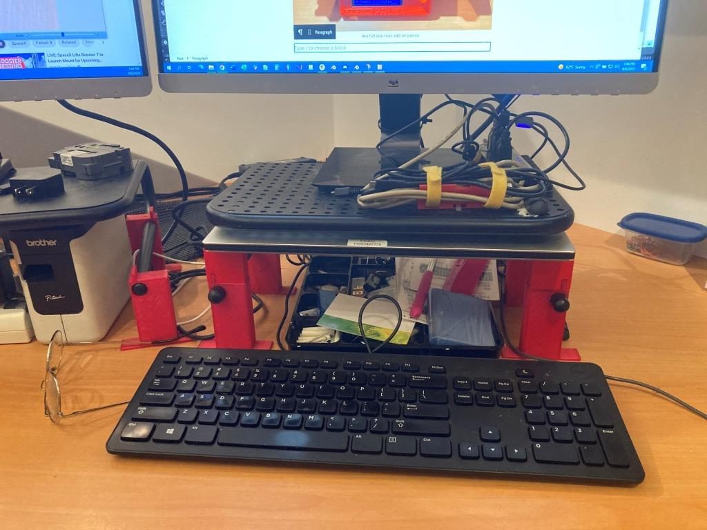
Jonathan encourages his students to go beyond the lessons and to modify or extend the particular focus of any lesson, so I decided to try and use Blender/CAD Sketcher for a small project I have been considering. My main PC is a Dell XPS15 laptop, connected to two 24″ monitors via a Dell WD19TBS Thunderbolt docking station. I have the monitors on 4″ risers, but found they still weren’t high enough for comfortable viewing and seating ergonomics, so I designed (in TCAD, several years ago) a set of riser risers as shown in the image below

My two-display setup. Note the red ‘riser elevators’ under the metal display risers
Closeup showing the built-in shelf for my XPS 15 laptop

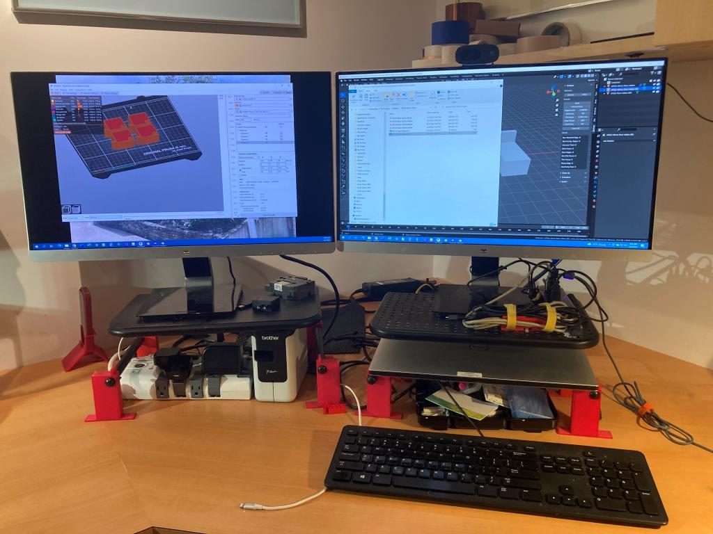
As shown above, the ‘riser elevator design incorporates a built-in shelf for my XPS15 laptop. This has worked well for years, but recently I have been looking for ways to simplify/neaten up my workspace. I found that I could move my junk tray from the side of my work area to the currently unused space underneath my laptop, but with the current arrangement there isn’t enough clearance above the tray to see/access the stuff in the back. I was originally thinking of simply replacing the current 3D printed risers with new ones 40mm higher, but in an ‘aha!’ moment I realized I didn’t have to replace the risers – I could simply add another riser on top. The new piece would mate with the current riser vertical tab that keeps the laptop from sliding sideways, and then replicate the same vertical tab, but 40mm higher.

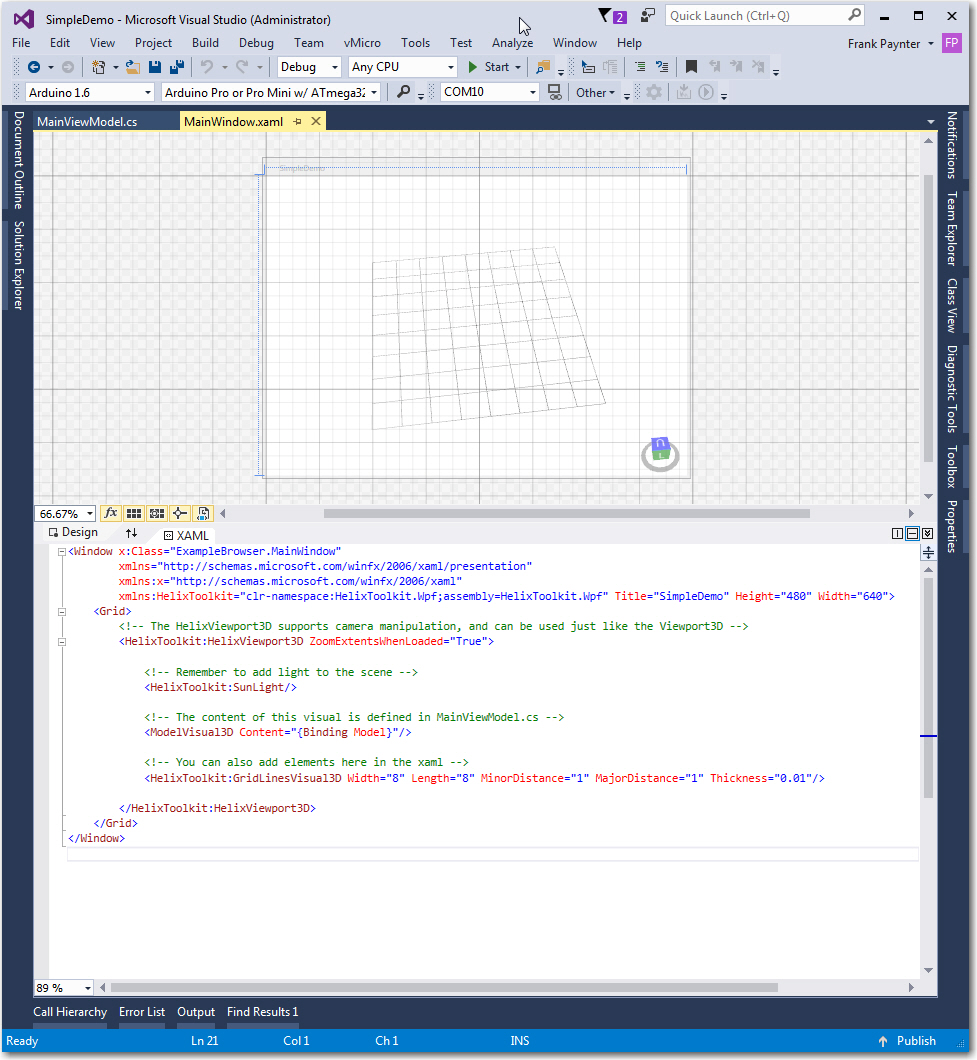
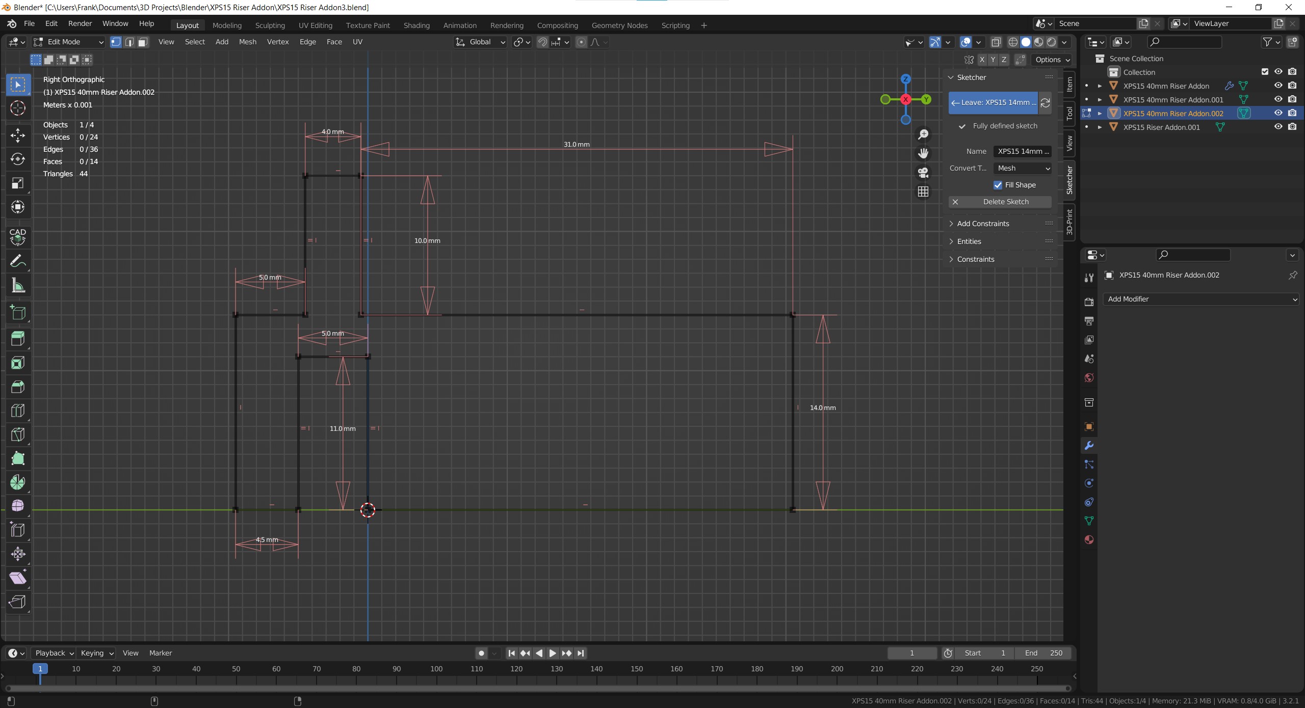
Doing either the re-designed riser or the add-on would be trivial in TinkerCad, but I thought it would be a good project to try in Blender, now that I have some small inkling of what I’m doing there. So, after the normal number of screwups, I came up with a fully-defined sketch for a small test piece (I fully subscribe to Jonathan’s “When in doubt – test it out” philosophy), as shown:

CAD Sketcher sketch for the test piece. Same as the final piece, except for height

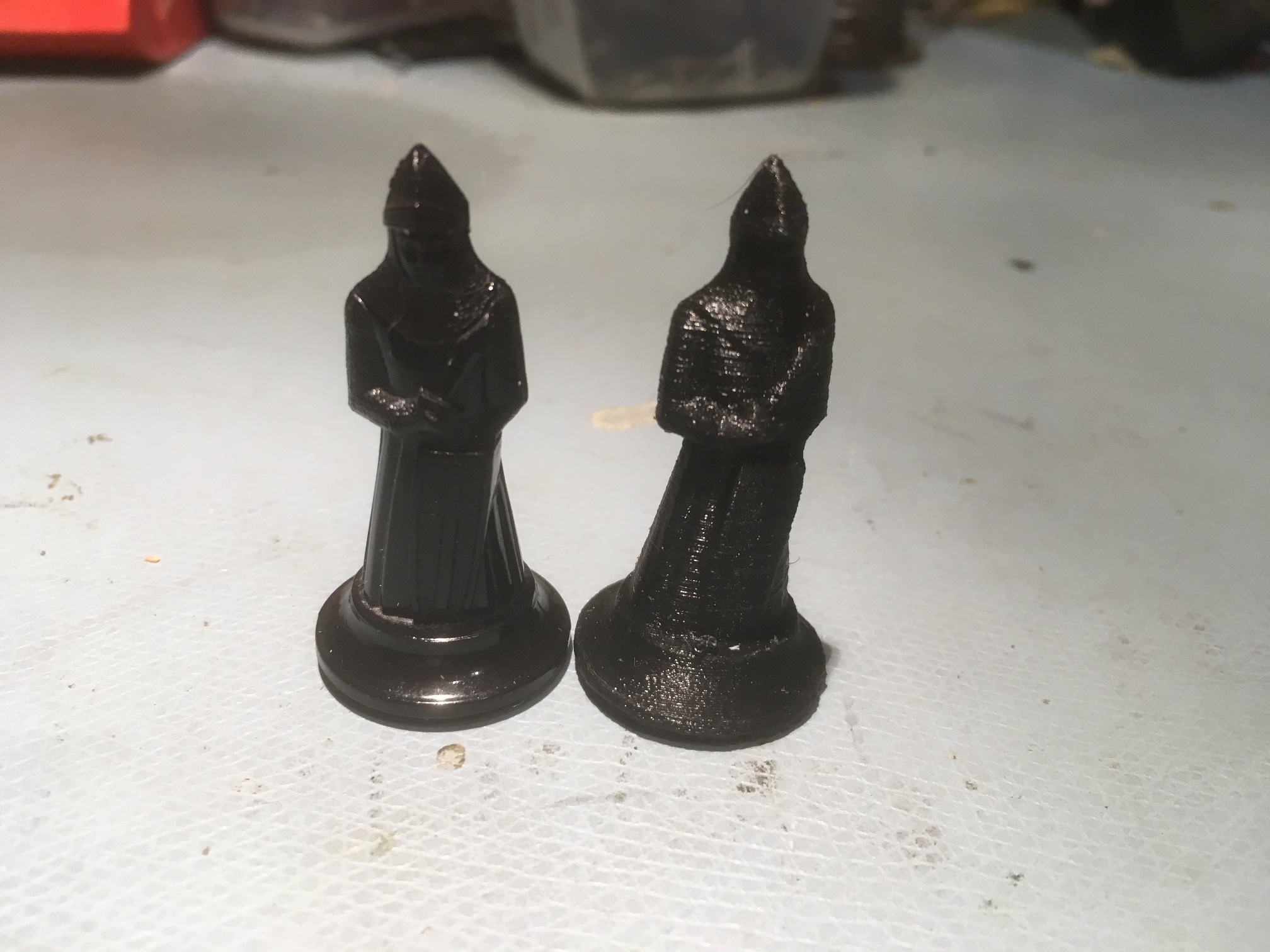
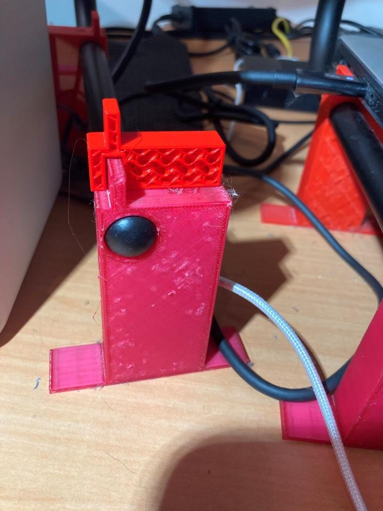
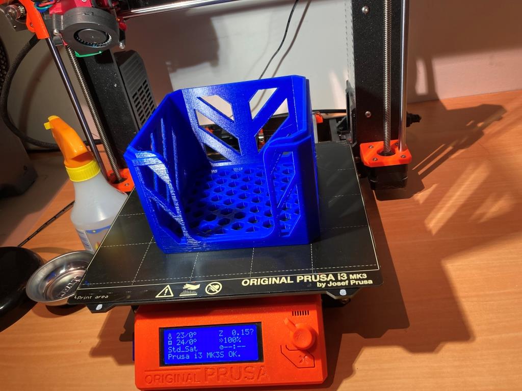
I then 3D printed on my Prusa MK3S printer. Halfway through the print job I realized I didn’t need the full 20mm thickness to test the geometry, so I stopped it midway through and placed it on top of one of the original risers, as shown in the following photo:

Maybe not completely perfect, but still a pretty good fit

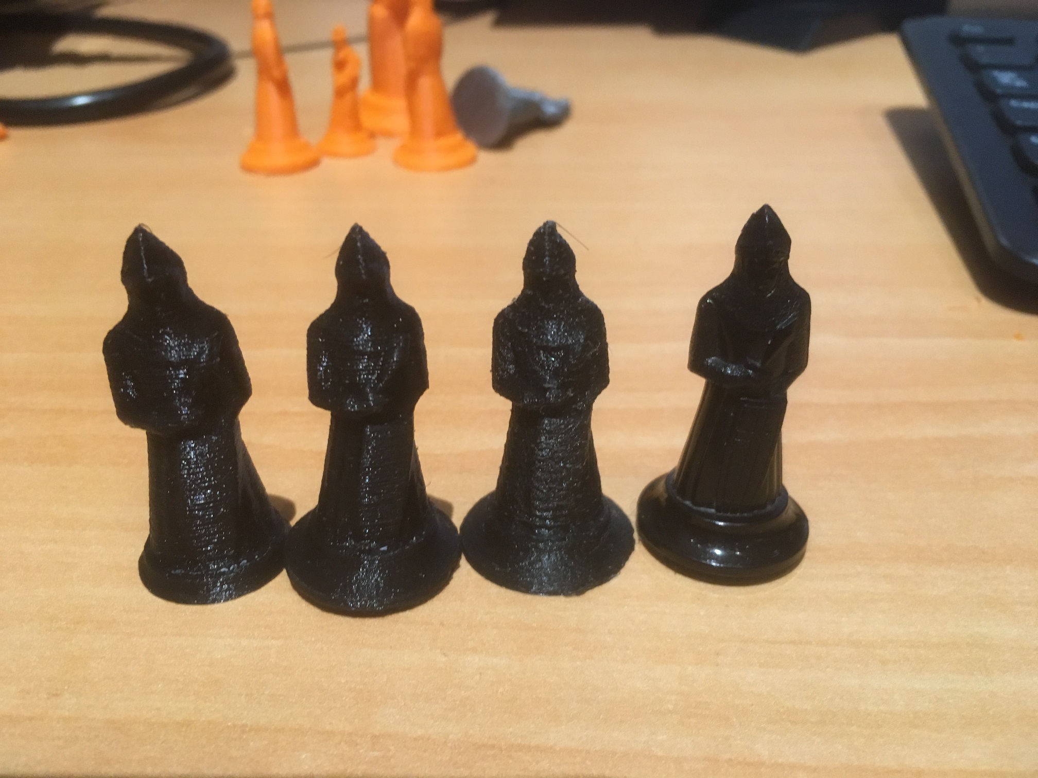
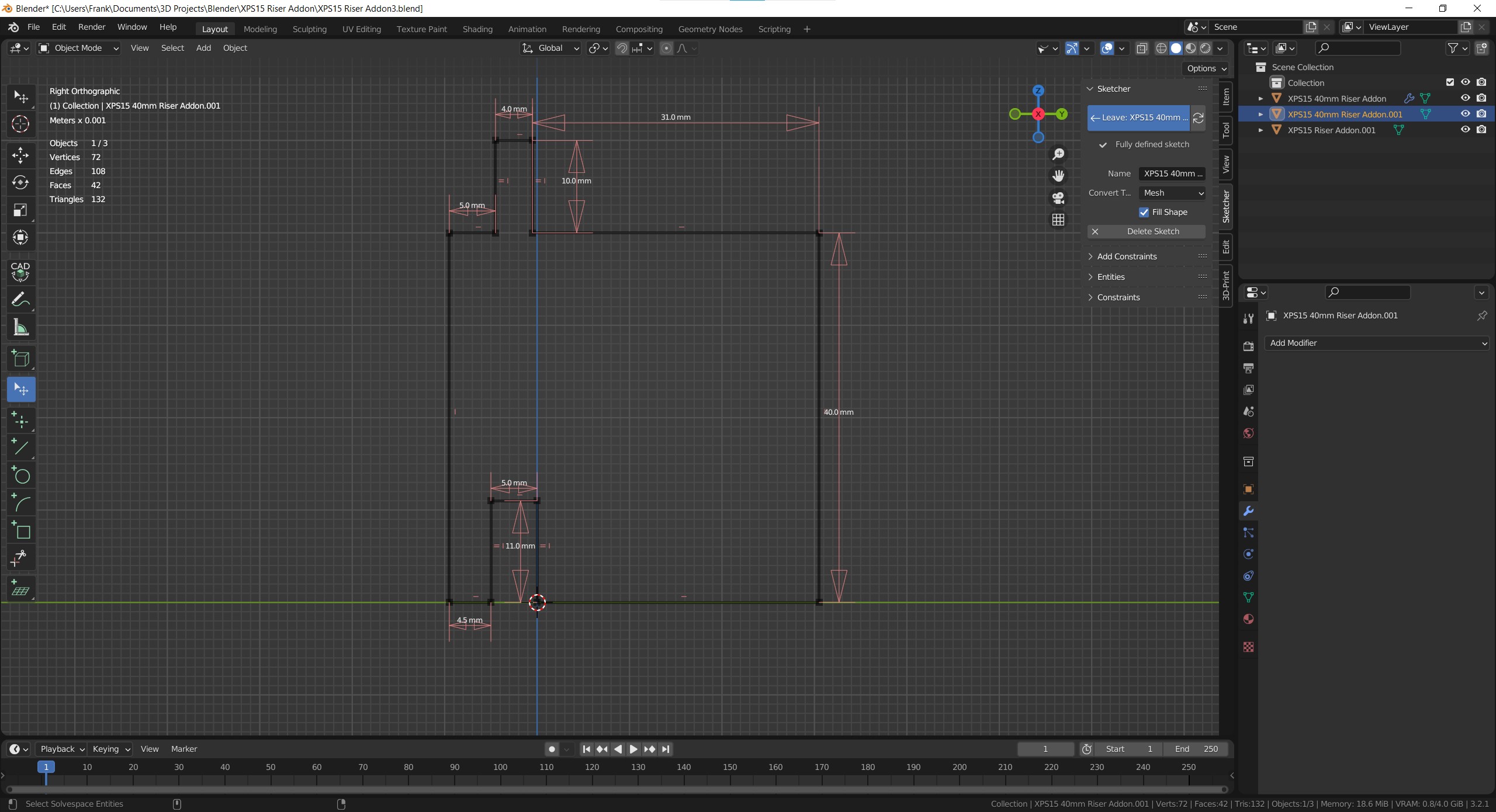
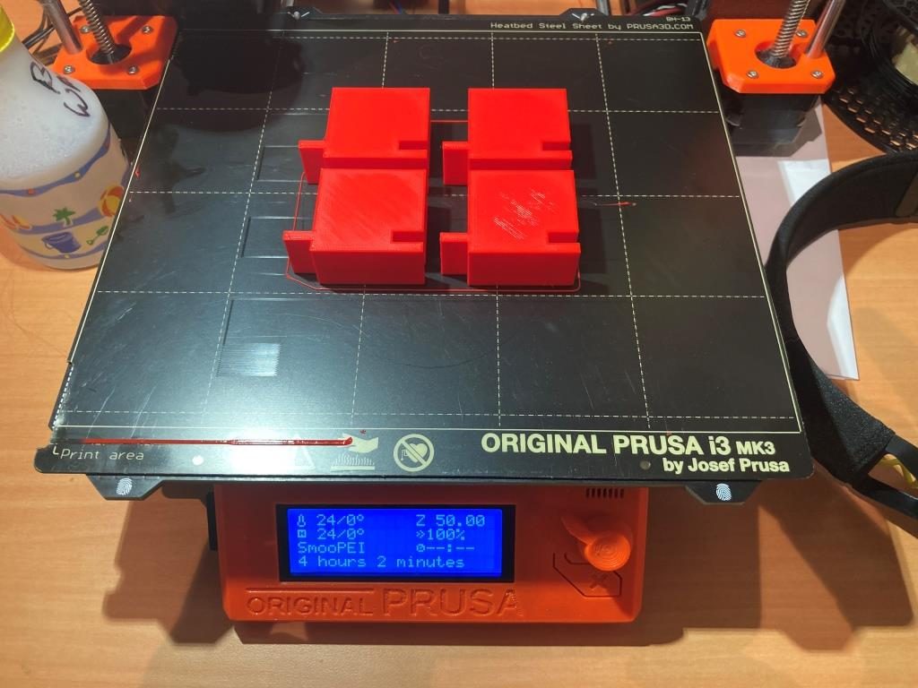
After convincing myself that the design was going to work, I modified the sketch for the full 40mm height I wanted, and printed 4ea out, as shown:

CAD Sketcher sketch for the full-height version
4ea full-size riser add-on pieces

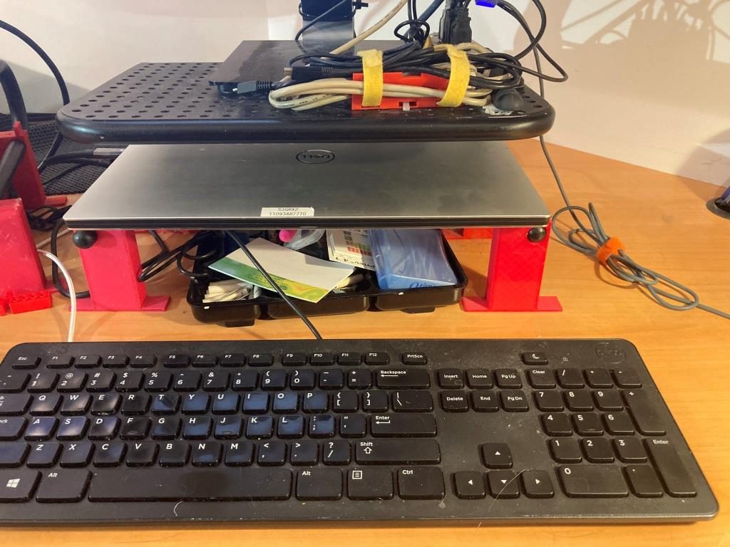
After installation, I now have my laptop higher by 40mm, and better/easier access to my junk tray as shown – success!

Finished project. Laptop higher by 40mm, junk tray now much more accessible

And more than that, I have now developed enough confidence in Blender/CAD Sketcher to move my 3D print designs there rather than relying strictly on TinkerCad. Thanks Jonathan!

16 August 2022 Update:

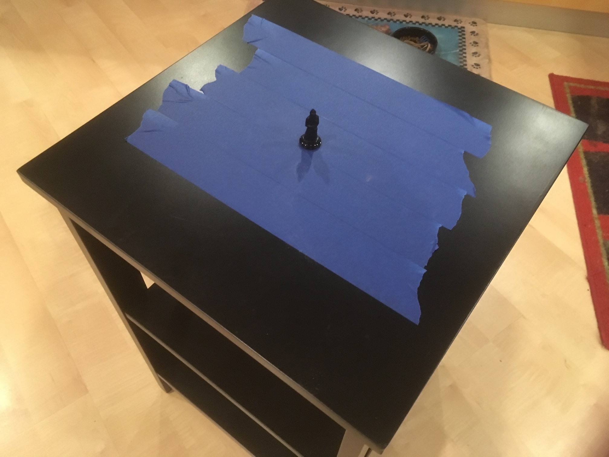
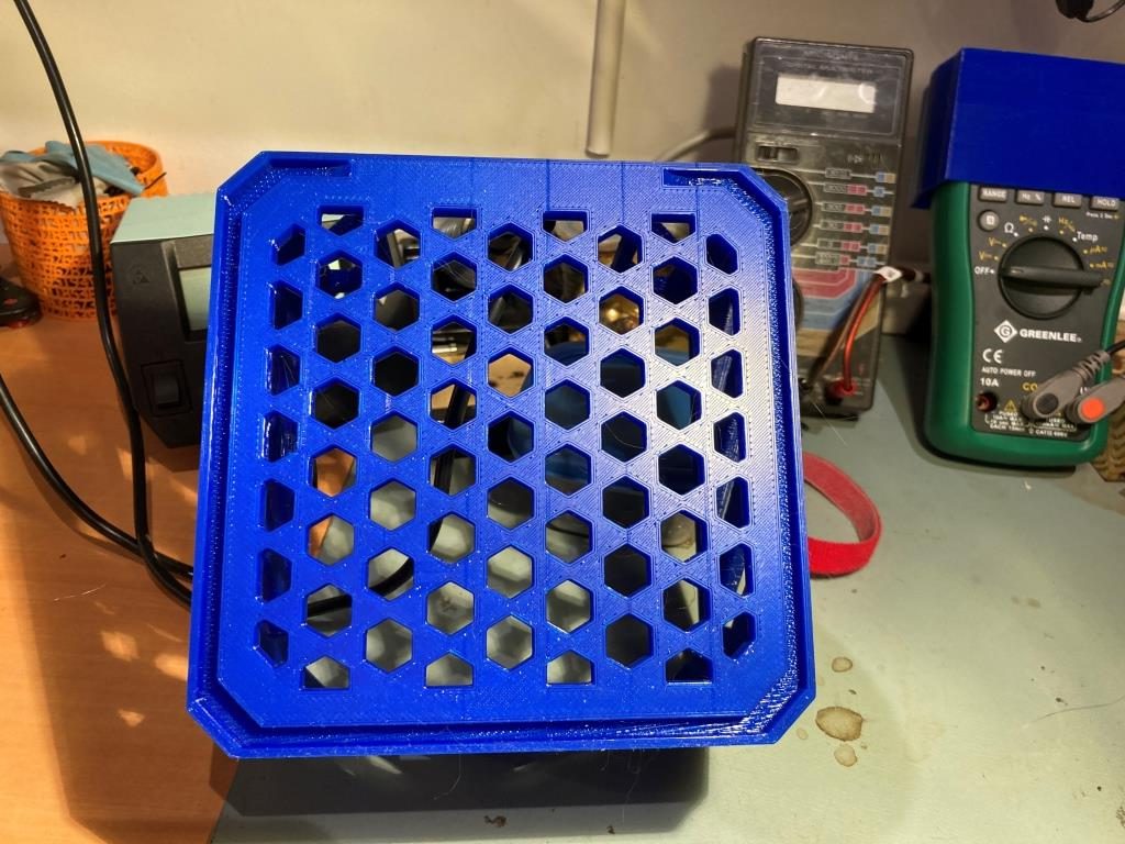
Just finished Learning Project 7: Stackable Storage Crate, and my brain is bulging at the seams – whew! After finishing, I just had to try printing one (or two, if I want to see whether or not I really got the nesting geometry right), even though each print is something over 13 hours on my Prusa MK3S with a 0.6mm nozzle. Here’s the result:

Hot off the printer – after “only” 13 hours!
Underside showing stacking groove. Printed without supports, just using bridging

Frank

New Wheels for Wall-E2

Posted 24 August 2020, 1402 days into the Covid-19 Lockdown

My autonomous wall-following robot Wall-E2 is now smart enough to reliably follow walls and connect to a charging station, at least in my office ‘sandbox’ testing area, as shown in the following video

However, as can be seen toward the end of the video, Wall-E2 had some trouble and almost got stuck making the third 90 degree turn.  Apparently the current thin 90mm wheels just don’t provide enough traction on carpet.

So, I decided to see what I could do about re-wheeling Wall-E2.  After some research I found there are now plenty of larger diameter wheels for robots out there, but I couldn’t seem to find a set that would fit Wall-E2 and still allow me to keep the current set of wheel guards.  I needed the same (or maybe slightly larger) diameter for ‘road’ clearance, but something less than about 20 mm thick to fit within the current wheel guard dimensions. Then it occurred to me while reading the specs for one of the wheels (ABS for the wheel, and TPU for the tire)  that I already had two 3D printers standing around waiting for something to do, and I had a plentiful supply of ABS (or in my case, PETG) and TPU filaments – why not build my own?  After all, how hard could it be?  As you might guess, that question started what now feels like a 10-year slog through ‘3D printed wheel hell’

I wanted to create a spoked wheel with a hub that would accept a 3mm flatted motor shaft, and I wanted to fit this wheel with a simple TPU treaded tire.  The wheel would have small ‘guard rail’ rims that would keep the tire from sliding off.

It started innocently enough with a search through Thingiverse, where I found several SCAD scripts for ‘parameterized’ wheels.  Great – just what the doctor ordered!  Well, except that the scripts, which may have worked fine for the authors, didn’t do what I wanted.  and as soon as I tried to adjust them to fit my design specs, I discovered they were incomplete, buggy, or both.

I had wanted to learn a bit more about SCAD anyway and this seemed like a good project to do that with, so I persevered, and eventually came up with a SCAD design that I liked.

I started with bioconcave’s ‘Highly Modular Wheel_v1.0.scad’ file from Thingiverse, and (after what seemed like years trying to understand what was going on) was able to extract modular pieces into my own ‘FlatTireWheel’ scad script, as follows:

Here’s a screenshot of a completed 86mm wheel with elliptical spokes and a hub compatible with a 3mm flatted shaft.  When a TPU tire is added to the rim, the assembly should be about 90mm in diameter.

SCAD-generated wheel with elliptical spokes and a hub compatible with a 3mm flatted shaft. Note extensions to set screw hole through spoke and rim

One of the many issues I had with the original code is it assumed the hub would sit on top of the spokes, and therefore there was no need to worry about whether or not the setscrew arrangement would be blocked by the spokes and/or rim.  Since I wanted a wheel that was mostly tread, I wanted to ‘sink’ the hub into the spokes as shown above. In order to make this work, I needed to extend the setscrew access hole through the spoke assembly and through the rim.  In the finished design, the hub assembly can be moved freely up and down in the center of the wheel, and the hole extensions will follow.  If the hub setscrew hole isn’t blocked by the spokes and/or rim, then the extensions don’t do anything; otherwise they extend the setscrew hole as shown above.

Here’s a photo of separate wheel/tire pieces, and a completed wheel/tire combination on Wall-E2

Separate wheel & tire parts, plus a completed wheel on Wall-E2

2 September 2020 Update:

After running some sandbox tests with my new wheels, I discovered that the new tires didn’t have much more traction than the old ones. However, now that I ‘had the technology’, it was a fairly simple task to design and print new tires to fit onto the existing new rims. Rather than do the tire design in SCAD, I found it much much easier to do this in TinkerCad. Here’s a couple of screenshots showing the TCad design.

Original printed tire on the left, new one on the right. Note more aggressive tread on new tire
Exploded view showing construction technique used for new (and old) tire. Very easy to do in TinkerCad!

03 September 2020 Update:

The increased traction provided by the new tires have caused a new problem; on a hard surface the rotation during a ‘spin turn’ (one side’s motors going forward, the other going in reverse) is too fast, causing the robot to slide well past the target heading. Not so much of a problem on carpet, but how would the robot know which surface is in play at the moment. After some thought, I decided to try and modulate the turn rate, in deg/sec, as a proxy for the surface type. So, in ‘SpinTurn()’ I put in some code to monitor the turn rate and adjust the motor speeds upward or downward to try and keep the turn rate at a reasonable level.

Here’s a video of a recent run utilizing the new ‘SpinTurn’ rate modulation algorithm

And the data from the three ‘spin turn’ executions, one on hard surface, and two on carpet.

Spin Turn executions; hard surface, followed by two carpet turns

As can be seen in the above video and plots, the motor speeds used on the hard surface turn is much lower than the speeds used during the carpet turns, as would be expected. This is a much nicer result than the ‘fire and forget’ algorithm used before. Moreover, the carpet turns are much more positive now thanks to the more aggressive tread on the new tires – yay!

Alzheimer’s Light Strobe Therapy Project

Posted 24 March, 2019

A friend told me about a recent medical study at MIT where lab mice (genetically engineered to form amyloid plaques in their brains to emulate a syndrome commonly associated with Alzheimer’s) were subjected a 40Hz strobe light several hours per day.  After repeated exposures, the mice showed significantly reduced plaque density in their brains, leading the researchers to speculate that ‘light strobe therapy’ might be an effective treatment for Alzheimer’s in humans.

The friend’s spouse has been diagnosed with Alzheimer’s, so naturally he was keen to try this with his spouse, and asked me if I knew anything about strobe lights and strobe timing, etc.  I told him I could probably come up with something fairly quickly, and so I started a project to design and fabricate a light strobe therapy box.

The project involves a 3D printed housing and 9V battery clip, along with a white LED and a Sparkfun Pro Micro 5V/16MHz microcontroller, as shown in the following schematic.

Strobe Therapy schematic

I had a reflector hanging around from another project, so I used it just as much for the aesthetics as for functionality, and I designed and printed up a 2-part cylindrical housing. I also downloaded and printed a 9V battery clip to hold the battery, as shown in the following photos

Finished Strobe Therapy Unit

Internal parts arrangement

Closeup showing Sparkfun Pro Micro microcontroller

The program to generate the 40Hz strobe pulses is simplicity itself.  I used the Arduino ‘elapsedMillis’ library for more accurate frequency tuning, but ‘delay()’ would probably be close enough as well.


I’m not sure if this will do any good, but I was happy to help someone whose loved one is suffering from this cruel disease.

Frank


Chess Piece Replacement Project

Posted 15 March 2019,

A week or so ago a family friend asked if I could print up a replacement part for a chess set.  I wasn’t sure I could, but what the heck – I told them to send it to me and I would do my best.  Some time later a package arrived with the piece (shown below) to be duplicated – a pawn I think.

Chess piece to be duplicated

Chess piece to be duplicated

The piece is about 43 x 20 x 20 mm, and as can be seen in the above photos, has a LOT of detail.  I didn’t know how close I could come, but I was determined to give it the old college try!

3D Scanning:

The first step was to create a 3D model of the piece.  I was semi-successful in doing something similar with an aircraft joystick about five years ago, but that piece was a lot bigger, and had a lot less detailed surface.   This previous effort was done using Autodesk Capture123, and it was a real PITA to get everything right.  Surely there were better options now?

My first thought was to utilize a professional 3D scanning service, but this turned out to be a lot harder than I thought. There is a LOT of 3D scanning hardware out there now, but most of it is oriented toward 3D scans of industrial plants, architecture installations and big machinery.  Very little to be found in the way of low-cost high-resolution 3D scanning hardware or services.  There are, of course, several hobbyist/maker 3D scanners out there, but the reviews are not very spectacular.  I did find two services that would scan my piece, but both would charge several hundred dollars for the project, and of course would require a round-trip mailing of the part itself – bummer.

Next, I started researching possibilities for creating a scan from photos – basically the same technique I used for the joystick project.  While doing this, I ran across the ‘Photogrammetry’ and ‘Photogrammetry 2’ video/articles produced by Prusa Research, the same folks who make the Prusa Mk3 printer I have in my lab – cool!  Reading through the article and watching the video convinced me that I had a shot at creating the 3D model using the Meshroom/AliceVision photogrammetry tool.

At first I tried to use my iphone 4S camera with the  chess piece sitting on a cardboard box for the input to Meshroom, but this turned out to be a disaster.  As the article mentioned, glossy objects, especially small black glossy objects, are not good candidates for 3D photogrammetry.  Predictably, the results were less than stellar.

Next I tried using my wife’s older but still quite capable Canon SX260 HX digital camera.  This worked quite a bit better, but the glossy reflectivity of the chess piece was still a problem. The wife suggested we try coating the model with baby powder, and this worked MUCH better, as shown in the following photos.  In addition, I placed the piece on a small end table covered with blue painter’s tape so I would have a consistent, non-glossy background for the photos.  I placed the end table in our kitchen so I could roll my computer chair around the table, allowing me to take good close-up photos from all angles.

End table covered with blue painter’s tape

Chess piece dusted with baby powder

Chess piece dusted with baby powder

Chess piece dusted with baby powder

Next, I had to figure out how to use Meshroom, and this was both very easy and very hard.  The UI for Meshroom is very nice, but there is next to no documentation on how to use it.  Drag and drop a folder’s worth of photos, hit the START button, and pray.

Meshroom UI

As usual (at least for me), prayer was not an effective strategy, as the process crashed or hung up multiple times in multiple places in the 11 step processing chain.  This was very frustrating as although voluminous log files are produced for each, the logs aren’t very understandable, and I wasn’t able to find much in the way of documentation to help me out.  Eventually I stumbled onto a hidden menu item in the UI that showed the ‘image ID’ for each of the images being processed, and this allowed me to figure out which photo caused the system to hang up.

Meshroom UI showing hidden ‘Display View ID’s’ menu item.

Once I figured out how to link the view ID shown in the log at the point of the crash/hangup with an actual photograph, I was able to see the problem – the image in question was blurred to the point where Meshroom/AliceVision couldn’t figure out how it fit in with the others, so it basically punted.

Photo that caused Meshroom/AliceVision to hang up

So, now that I had some idea what was going on, I went through all 100+ photos looking for blurring that might cause Meshroom to hang up.  I found  and removed five more that were questionable, and after doing this, Meshroom completed the entire process successfully – yay!!

After stumbling around a bit more, I figured out how to double-click on the ‘Texturing’ block to display the solid and/or textured result in the right-hand model window, as shown in the following photo, with the final solid model oriented to mirror the photo in the left-hand window.

textured model in the right-hand window oriented to mirror the photo in the left-hand window

So, the next step (I thought) was to import the 3D .obj or .3MF file into TinkerCad, clean up the artifacts from the scanning process, and then print it on my Prusa Mk3.  Except, as it turns out, TinkerCad has a 25MB limit on imports due to its cloud-based nature, and these files are way bigger than 25MB – oops!

Back to the drawing board; first I looked around for an app I could use to down-size the .obj file to 25MB so it would fit into TinkerCad, but I couldn’t figure out how to make anything work.  Then I stumbled across the free Microsoft suite of apps for 3D file management – 3DPrint, 3DView, and 3DBuilder.  Turns out the 3DBuilder app is just what the doctor ordered – it will inhale the 88MB texturedMesh.obj file from Meshroom without even breaking a sweat, and has the tools I needed to remove the scanning artifacts and produce a 3MF file, as shown in the following screenshots.

.OBJ file from Meshroom after drag/drop into Microsoft 3DBuilder. Note the convenient and effective ‘Repair’ operation to close off the bottom of the hollow chess piece

Side view showing all the scanning artifacts

View showing all the disconnected scanning artifacts selected – these can be deleted, but the other artifacts are all connected to the chess piece

The remaining artifacts and chess piece rotated so the base plane is parallel to the coordinate plane, so it can be sliced away

Slicing plane adjusted to slice away the base plane

After the slicing operation, the rest of the scanning artifacts can be selected and then deleted

After all the scanning artifacts have been cleared away

Chess piece reoriented to upright position

Finished object exported as a .3MF file that can be imported into Slic3r PE

Now that I had a 3D object file representing the chess piece, I simply dropped it into Slic3r Prusa Edition, and voila! I was (almost) ready to print!  In Slic3r, I made the normal printing adjustments, and started printing trial copies of the chess piece.  As usual I got the initial scale wrong, so I had to go through the process of getting this right.  In the process though, I gained some valuable information about how well (or poorly) the 3D scan-to-model process worked, and what I could maybe improve going forward.  As shown in the following photo, the first couple of trials, in orange ABS, were pretty far out of scale (original model in the middle)

I went through a bunch of trials, switching to gray and then black PLA, and narrowing the scale down to the correct-ish value in the process.

The next photo is a detail of the 4 right-most figures from the above photo; the original chess piece is second to right.  As can be seen from the photo, I’m getting close!

All of the above trials were printed on my Prusa Mk3 using either orange ABS or gray (and then black) PLA, using Prusa’s preset for 0.1mm layer height.  Some with, and some without support.

After the above trials, I went back through the whole process, starting with the original set of scan photos, through Meshroom and Microsoft 3D Builder to see if I could improve the 3D object slightly, and then reprinted it using Prusa’s 0.05mm ‘High Detail’ settings.  The result, shown in the following photos is better, but not a whole lot better than the 0.1mm regular ‘Detail’ setting.

Three of the best prints, with the original for comparison. The second from right print is the 0.05mm ‘super detail’ print

I noticed that the last model printed was missing part of the base – a side effect of the slicing process used to remove scanning artifacts.  I was able to restore some of the base in 3D Builder using the ‘extrude down’ feature, and then reprinted it. The result is shown in the photo below.


“Final” print using Prusa Mk3 with generic PLA, Slic3r PE with 0.1mm ‘Detail’ presets, with support

Just as an aside, it occurred to me at some point that the combination of practical 3D scanning using a common digital camera and practical 3D printing using common 3D printers is essentially the ‘replicator’ found in many Sci-Fi movies and stories.  I would never thought that I would live to see the day that sci-fi replicators became reality, but at least in some sense it has!

Stay tuned!

Frank


Magnetometer Calibration Tool, Part IV

In my  last episode of the Magnetometer Calibration Tool soap opera, I had a ‘working’ WPF application that could be used to generate a 3×3 calibration matrix and 3D center offset value for any magnetometer capable of producing  3D magnetometer values  via a serial port.  Although the tool worked, it had a couple of ‘minor’ deficiencies:

  • My original Eyeshot-based tool sported a very nice set of 3D reference circles in both the ‘raw’ and ‘calibrated viewports.  In the ‘raw’ view, the circle radii were equal to the average 3D distance of all  point cloud points from the center, and in the ‘calibrated’ view the circle radii were exactly 1.  This allowed the user to readily visualize any deviations from ideal in the ‘raw’ view, and the (hopefully positive) effect of the calibration algorithm.  This feature was missing from the WPF-based tool, mainly because I couldn’t figure out how to do it :-(.
  • The XAML and ‘code-behind’ associated with the project was a god-awful mess!  I had tried lots and lots of different things while blindly stumbling toward a ‘mostly working’ solution, and there was a  LOT of dead code and inappropriate structure still hanging around.  In addition to being ugly, this state of affairs also reflected my (lack of) understanding of basic WPF/Helix Toolkit concepts, principles, and methods.

So, this post describes my attempts to rectify both of these problems.  Happily, I can report that the first one (lack of switchable reference circles) has been completely solved, and the second one (god-awful mess and lack of understanding) has been at least partially rectified; I have a much better (although not complete by any means!) grasp of how XAML and ‘code-behind’ works together to produce the required visual effects.

To achieve better understanding of the connection between the 3D viewport implemented in Helix Toolkit by the HelixViewport3D object, the XAML that describes the window’s layout, and the ‘code-behind’ C# code, I spent a lot of quality time working with and modifying the Helix Toolkit’s ‘Simple Demo’ app.  The ‘Simple Demo’ program displays 3 box-like objects (with some spheres I added) on a grid, as shown below

Simple Demo WPF/Helix Toolkit Application

Simple Demo WPF/Helix Toolkit Application (spheres added by me)

Simple Demo XAML View

Simple Demo XAML View – no changes from original

Simple Demo 'Code-behind', with my addition highlighted

Simple Demo ‘Code-behind’, with my addition highlighted

My aim in going back to the ‘Simple Demo’ was to avoid  the distraction of my more complex window layout (2 separate HelixViewport3D windows and  lots of other controls) and the associated C#/.NET code so I could concentrate on one simple task – how to  implement a set of 3D reference circles that can be switched on/off via a windows control (a checkbox in my case).  After trying a lot of different things, and with some clues garnered from the Helix Toolkit forum, I settled on the TubeVisual3D object to construct the circles, as shown in the following screenshots.  I used an empirically determined ‘thickness factor’ of 0.05*Radius for the ‘Diameter’ property to get the ‘thick circular line’ effect I wanted.

Simple Demo modified to implement TubeVisual3D objects

Simple Demo modified to implement TubeVisual3D objects.  The original box/sphere stuff is still there, just too small to see

MyWPFSimpleDemo 'code-behind', with TubeVisual3D implementation code highlighted

MyWPFSimpleDemo ‘code-behind’, with TubeVisual3D implementation code highlighted.  Note all the ‘dead’ code where I tried to use the EllipsoidVisual3D model for this task.

Next, I had to figure out a way of switching the reference circle display on and off using a windows control of some sort, and this turned out to be frustratingly difficult.  It was easy to get the circles to show up on program startup – i.e. with model construction and the connection to the viewport established in the constructor(s), but I could not figure out a way of doing the same thing after the program was already running.  I knew this had to be easy – but damned if I could figure it out!  Moreover, after hours of searching the blogosphere, I couldn’t find anything more than a few hints about how to do it. What I  did find was a lot of WPF beginners like me with the same problem but no solutions – RATS!!

Finally I twigged to the fundamental concept of WPF 3D visualization – the connection between a WPF viewport (the 2D representation of the desired  3D model) and the ‘code-behind’ code that actually represents the 3D entities to be displayed must be defined at program startup, via the following constructs:

  • In the XAML, a line like  ‘<ModelVisual3D Content=”{Binding Model}”/>, where Model is the name of a  Model3D property declared in the  ‘code-behind’ file (MainViewModel.cs in my case)
  • In MainWindow.xaml.cs, a  line like ‘this.DataContext = mainviewmodel’, where mainviewmodel is declared with ‘public MainViewModel mainviewmodel = new MainViewModel();’
  • In MainViewModel.cs, a line like ‘ public Model3D Model { get; set; }’, and in the class constructor, ‘Model = new Model3DGroup();’
  •  in MainViewModel.cs, the line ‘var modelGroup = new Model3DGroup();’ at the top of the model creation section to create a temporary Model3DGroup object, and the line ‘ this.Model = modelGroup;’ at the bottom of the model construction code. This line sets the Model property contents to the contents of the temporary modelGroup‘ object

So, the ‘MainViewModel’ class is connected to the Windows window  class in MainWindow.xaml.cs, and the 3D model described in the MainViewModel class is connected to the 3D viewport via the Model Model3DGroup object.  This is all done at initial object construction, in the various class constructors.  There are still some parts of this that I do not understand, but I think I have it mostly correct.

The important concept that I was missing  is the above connections have been made at program startup and cannot (AFAICT) be changed once the program starts, but the contents of the temporary  Model3DGroup object (i.e. the ‘Children’ objects in the model group) can be changed, and the new contents will be reflected in the viewport when it is next updated.  Once I understood this concept, the rest, as they say, “was history”.  I implemented a simple control handler that cleared the contents of the temporary Model3DGroup object modelGroup and regenerated it (or not, depending on the state of the ‘Show Ref Circles’ checkbox).  Simple and straightforward, once I knew the secret!

So this ‘aha’ moment allowed me to implement the switchable reference circles in my Magnetometer calibration tool and check off the first of the deficiencies noted at the start of this post.  The new reference circle magic is shown in the following screenshots.

Raw and calibrated magnetometer data. Calculated average radius of the raw data is about 444 units, and the assumed average radius of the calibrated data is close to 1 unit

Raw and calibrated magnetometer data. Calculated average radius of the raw data is about 444 units, and the assumed average radius of the calibrated data is close to 1 unit

Raw and calibrated magnetometer data, with reference circles shown. The radius of the 'raw' circles is equal to the calculated average radius of about 444 units, and the assumed average radius of the calibrated circles is exactly 1 unit

Raw and calibrated magnetometer data, with reference circles shown. The radius of the ‘raw’ circles is equal to the calculated average radius of about 444 units, and the assumed average radius of the calibrated circles is exactly 1 unit

The reference circles make it easy to see how the calibration process affects the data.  In the ‘raw’ view, it is apparent that the data is significantly offset from center, but still reasonably spherical.  In the calibrated view, it is easy to see that the calibration process centers the data, removes most of the non-sphericity, and scales everything to very nearly 1 unit – nice!

Now for addressing the second of the two major deficiencies noted at the start of this post, namely “The XAML and ‘code-behind’ associated with the project was a god-awful mess! “.

With my current understanding of a typical WPF-based application, I believe the application architecture consist of three parts – the XAML code (in MainWindow.xaml)    that describes the window layout,  the ‘MainWindow’ class (in MainWindow.cs) that contains the interaction logic with the main window, and a class or classes that generate the 3D models to be rendered in the main window.  For  my magnetometer calibration tool  I created  two 3D model generation classes – ViewportGeometryModel and RawViewModel.  The ViewportGeometry class is the base class for RawViewModel, and handles generation of the three orthogonal TubeVisual3D ‘circles.  The  ViewportGeometryModel class is instantiated directly (as ‘calmodel’ in the code) and connected to the main window’s ‘vp_cal’ HelixViewport3D window via it’s ‘GeometryModel’ Model3D property, and the derived class RawViewModel (instantiated in the code as ‘rawmodel’) is similarly connected to the main window’s ‘vp_raw’ HelixViewport3D window via the same  ‘GeometryModel’ Model3D property (different object instantiation, same property name).

The ViewportGeometryModel class has one main function, and some helper stuff.  The main function  is  ‘DrawRefCircles(HelixViewport3D viewport, double radius = 1, bool bEnable = false)’.  This function is called from MainWindow.xaml.cs as follows:

The ‘DrawRefCircles()’ function creates a new ModelGroup3D object if necessary, and optionally fills it with three TubeVisual3D objects of the desired radius and thickness, as shown below

The last line in the above function is ‘GeometryModel = modelGroup;’, where ‘GeometryModel’ is declared in the ViewGeometryModel class as

and bound to the appropriate HelixViewport3D window via

Line in MainWindow.xaml that binds the HelixViewport3D to the 'GeometryModel' Model 3D property of the ViewportGeometryModel class

Line in MainWindow.xaml that binds the HelixViewport3D to the ‘GeometryModel’ Model 3D property of the ViewportGeometryModel class (and/or its derived class RawViewModel). The line shown here is for the raw viewport, and there is an identical one in the calibrated viewport section.

Now, instead of a mishmash spaghetti factory, the program is a lot more organized, modular, and cohesive (or at least I think so!).  As the following screenshot shows, there are only a few classes, and each class does a single thing.  Mission accomplished!

Magnetometer calibration tool class diagram. Note that the RawViewModel is a derived class from VieportGeometryModel

Magnetometer calibration tool class diagram. Note that the RawViewModel is a derived class from VieportGeometryModel.  The ViewportGeometryModel.CirclePlane ‘class is an Enum

Other Stuff:

This entire post has been a description of how I figured out the connections between a WPF-based windowed application with two HelixViewport3D 3D viewports (and lots of other controls) and the XAML/code-behind elements that generate the 3D models to be rendered. In particular it has been a description of the ‘reference circle’ feature for both the ‘raw’ and ‘calibrated’ views.  However, these circles are really only a small part of the overall magnetometer calibration tool; a much bigger part of the 3D view are  the point-clouds in both the raw and calibrated views that depict the actual 3D magnetometer values acquired from the magnetometer being calibrated, before and after calibration.  I didn’t say anything about these point-cloud collections, because I had them working long before I started the ‘how can I display these damned reference circles’ odyssey.  However, I thought it might be useful to point out (no pun intended) some interesting tidbits about the point-cloud implementation.

  • I implemented the point-cloud using the Helix Toolkit’s PointsVisual3D and Point3DCollection objects.  Note that the PointsVisual3D object is derived from ScreenSpaceVisual3D which is derived from RenderingModelVisual3D  instead of a geometry object like TubeVisual3D which is derived from  ExtrudedVisual3D, which in turn is derived from  MeshElement3D.   These are very different inheritance chains.  A  PointsVisual3D object can be added directly to a HelixViewport3D object’s Children collection,  and doesn’t need a light for rendering!  I can’t tell you how much agony this caused me, as I just couldn’t understand why other objects added via the ModelGroup chain either didn’t render at all, or rendered as flat black objects.  Fortunately for me, the ‘SimpleDemo’ app  did have light already defined, so things displayed normally (it still took me a while to figure out that I had to add a light to my MagCal app, even though the point-cloud displayed fine).
  • Points in a point-cloud collection don’t support a ‘selected’ property, so I had to roll my own selection facility.  I did this by handling the mouse-down event, and manually checking the distance of each point in the collection from the mouse-down point.  If I found a point(s) close enough, I manually moved the point from the ‘normal’ point-cloud to a ‘selected’ point-cloud, which I rendered slightly larger and with a different color.  If a  point became ‘unselected’, I manually moved it back into the ‘normal’ point-cloud object.  A bit clunky, but it worked.

All of the source code, and a ZIP file containing everything (except Octave) needed to run the Magnetometer Calibration app is available at my GitHub site –  https://github.com/paynterf/MagCalTool

Frank