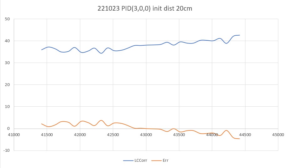
In TrackRightWallOffset with Kp/Ki/Kd = 300.00 0.00 10.00
In TrackRightWallOffset with RR/RC/RF = 30 30 30
straight window = 8 cm
R/C/F dists = 30 30 30 Steerval = 0.020, WallAngle = 1.14, Inside
In SpinTurn(CCW, 28.86, 45.00)
R/C/F dists = 27 30 30 Steerval = 0.350, WallOrientDeg = 20.00
approach start: orient angle = 20.000, tgt_distCm = 40
At start - err = prev_err = -10
R/C/F dists = 27 30 30 Steerval = 0.350, OrientDeg = 20.00, err/prev_err = -10
R/C/F dists = 27 30 30 Steerval = 0.350, OrientDeg = 20.00, err/prev_err = -10
Msec RFront RCtr RRear Orient Front Rear Err P_err
68368: Error in GetFrontDistCm() - 0 replaced with 60
68384 31 30 28 17.1 118 46 -10 -10
68496 34 33 30 22.3 125 56 -7 -10
68609 36 36 32 24.0 119 60 -4 -7
68720 39 38 34 28.0 115 66 -2 -4
68831 44 41 36 44.0 108 68 1 -2
At end of offset capture - prev_res*res = -2
correct back to parallel (Right side): RF/RC/RR/Orient = 44 41 36 44.00
In SpinTurn(CW, 44.00, 30.00)
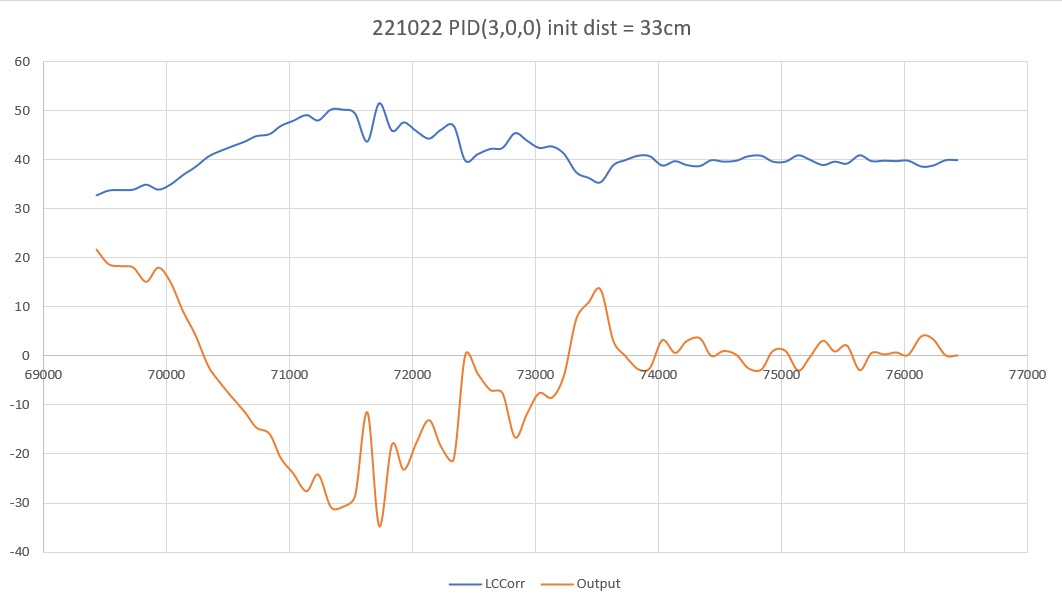
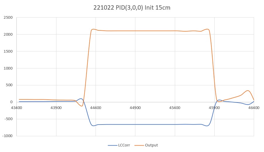
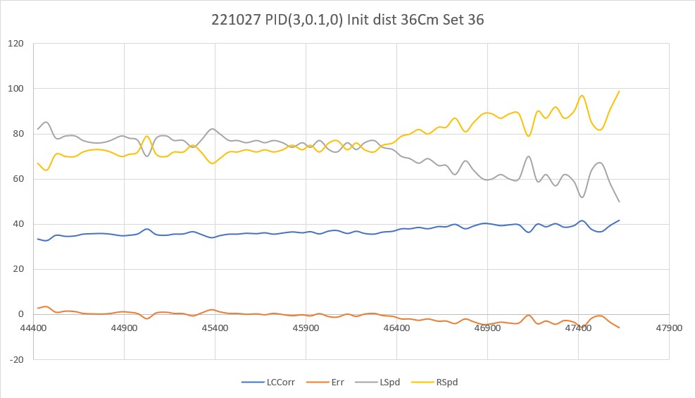
TrackRightWallOffset: Start tracking offset of 40.00cm with Kp/Ki/Kd = 300.00 0.00 10.00
Msec LF LC LR RF RC RR F Fvar R Rvar Steer Set Output LSpd RSpd
69557 728 794 816 49 47 50 95 10899 73 39363 -0.10 -0.07 8.70 66 83
69657 728 794 816 50 51 52 99 10901 80 39332 -0.18 -0.11 20.60 54 95
69756 728 794 816 50 48 50 93 10910 86 39318 0.00 -0.08 -22.50 97 52
69858 728 794 816 49 46 48 90 10917 94 39277 0.09 -0.06 -44.30 119 30
69958 728 794 816 46 44 47 86 10927 87 39265 -0.10 -0.04 15.90 59 90
70055 728 114 816 44 45 45 76 10956 102 39252 -0.11 -0.05 18.00 57 93
70157 728 108 816 43 41 43 77 10976 819 48383 -0.02 -0.01 3.50 71 78
70255 728 109 816 39 38 40 74 10994 123 48334 -0.09 0.02 32.00 43 107
70357 109 99 816 36 36 38 70 11023 750 55303 -0.19 0.04 67.80 7 127
70455 112 103 816 34 33 34 65 11056 104 55318 -0.02 0.07 28.40 46 103
70557 728 116 816 29 30 31 55 11101 819 63702 -0.15 0.10 73.40 1 127
70655 728 120 816 27 27 28 48 11170 106 63708 -0.08 0.13 63.40 11 127
70757 728 794 816 24 24 25 43 11246 110 63715 -0.11 0.15 77.50 0 127
70854 728 794 816 22 22 24 37 11329 118 55334 -0.19 0.15 101.20 0 127
In HandleAnomalousConditions with WALL_OFFSET_DIST_AHEAD error code detected
WALL_OFFSET_DIST_AHEAD case detected with tracking case Neither
In SpinTurn(CCW, 90.00, 45.00)
71682: glLeftCenterCm = 794 glRightCenterCm = 25
glLeftCenterCm > glRightCenterCm --> Calling TrackRightWallOffset()
71686: TrackRightWallOffset(), glRightFrontCm = 26
In TrackRightWallOffset with Kp/Ki/Kd = 300.00 0.00 10.00
In TrackRightWallOffset with RR/RC/RF = 26 25 26
straight window = 8 cm
R/C/F dists = 26 25 26 Steerval = -0.060, WallAngle = -3.43, Inside
In SpinTurn(CCW, 33.43, 45.00)
R/C/F dists = 26 30 32 Steerval = 0.610, WallOrientDeg = 34.86
approach start: orient angle = 34.857, tgt_distCm = 40
At start - err = prev_err = -8
R/C/F dists = 26 30 32 Steerval = 0.610, OrientDeg = 34.86, err/prev_err = -8
R/C/F dists = 27 33 33 Steerval = 0.580, OrientDeg = 33.14, err/prev_err = -8
Msec RFront RCtr RRear Orient Front Rear Err P_err
72138 33 33 27 33.1 219 25 -7 -8
72254 40 38 31 40.0 195 29 -3 -7
72365 44 43 34 43.4 187 32 3 -3
At end of offset capture - prev_res*res = -9
correct back to parallel (Right side): RF/RC/RR/Orient = 44 43 34 43.43
In SpinTurn(CW, 43.43, 30.00)
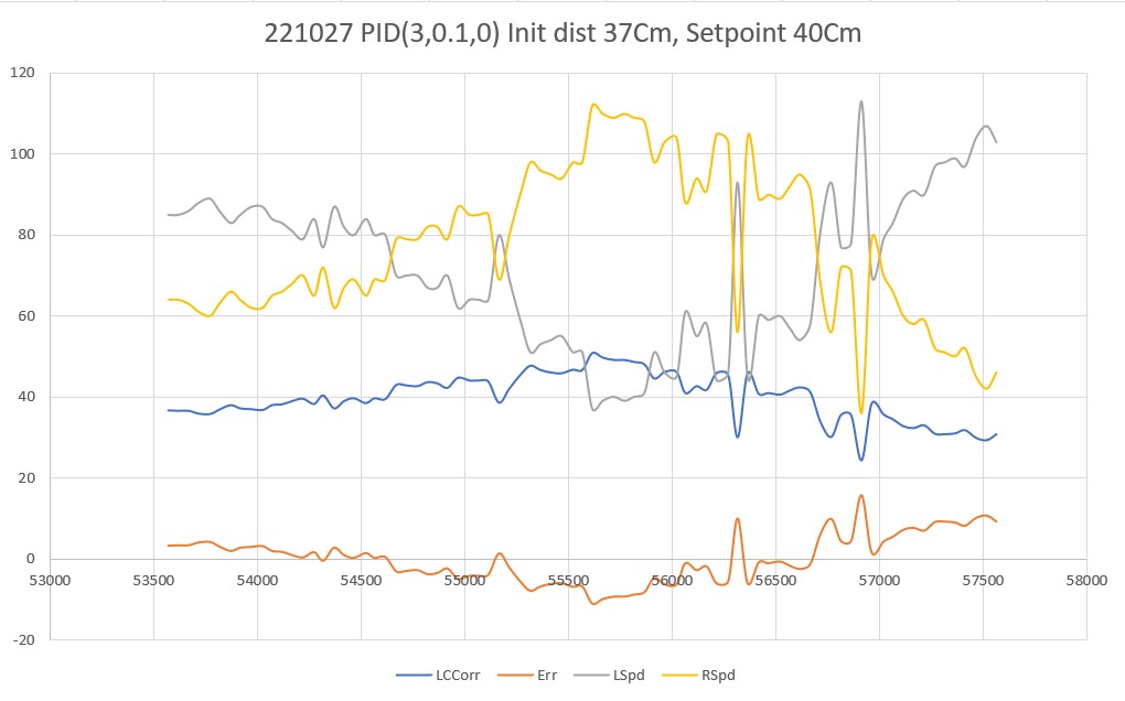
TrackRightWallOffset: Start tracking offset of 40.00cm with Kp/Ki/Kd = 300.00 0.00 10.00
Msec LF LC LR RF RC RR F Fvar R Rvar Steer Set Output LSpd RSpd
73091 110 112 122 40 38 39 151 11228 29 55621 0.09 0.02 -20.30 95 54
73189 728 110 816 39 40 41 153 11220 35 55688 -0.14 0.00 39.90 35 114
73291 728 112 816 40 38 39 150 11210 37 55762 0.18 0.02 -45.00 120 29
73394 728 111 816 40 38 39 146 11195 36 55854 0.06 0.02 -13.20 88 61
73492 114 115 120 38 37 38 141 11171 41 55917 0.07 0.03 -12.00 87 63
73589 728 113 816 38 38 38 134 11147 50 55921 -0.03 0.02 14.10 60 89
73692 728 116 816 36 37 36 129 11102 56 55913 0.05 0.03 -5.30 80 69
73789 112 115 816 36 35 36 124 11068 55 55971 0.00 0.05 14.30 60 89
73890 728 117 816 35 33 34 118 11028 64 56027 0.14 0.07 -19.80 94 55
73991 728 120 816 34 33 34 112 10988 69 56080 0.00 0.07 19.60 55 94
74090 728 120 816 34 33 32 109 10942 67 56165 0.11 0.07 -10.90 85 64
74189 728 122 816 33 32 32 103 10880 72 56246 0.06 0.08 5.40 69 80
74290 728 122 816 32 31 32 100 10825 85 56296 0.03 0.09 17.60 57 92
74393 728 794 816 32 30 31 92 10778 91 56321 0.10 0.10 0.60 74 75
74489 728 120 816 31 30 31 85 10736 86 56382 -0.01 0.10 31.90 43 106
74589 728 794 816 30 30 30 81 10687 92 56196 -0.01 0.10 33.00 42 108
74689 728 119 816 30 29 30 78 10611 104 56033 -0.01 0.11 35.90 39 110
74793 728 123 816 30 28 29 74 10519 107 55890 0.11 0.12 4.10 70 79
74890 728 122 816 30 29 29 71 10414 107 55749 0.12 0.11 -2.80 77 72
74990 728 794 816 31 29 29 67 10296 119 55629 0.20 0.11 -26.20 101 48
75089 728 115 816 31 30 29 63 10341 122 55523 0.15 0.10 -15.40 90 59
75189 728 119 816 31 31 30 59 10388 111 55452 0.09 0.09 -0.50 75 74
75290 728 115 816 32 31 30 52 10501 750 62042 0.20 0.09 -31.90 106 43
75392 728 119 816 33 31 30 47 10633 819 69966 0.30 0.09 -62.00 127 12
75490 728 123 816 32 32 31 40 10775 819 77492 0.12 0.08 -13.70 88 61
In HandleAnomalousConditions with WALL_OFFSET_DIST_AHEAD error code detected
WALL_OFFSET_DIST_AHEAD case detected with tracking case Neither
In SpinTurn(CCW, 90.00, 45.00)
76435: glLeftCenterCm = 794 glRightCenterCm = 26
glLeftCenterCm > glRightCenterCm --> Calling TrackRightWallOffset()
76440: TrackRightWallOffset(), glRightFrontCm = 27
In TrackRightWallOffset with Kp/Ki/Kd = 300.00 0.00 10.00
In TrackRightWallOffset with RR/RC/RF = 27 25 26
straight window = 8 cm
R/C/F dists = 27 25 26 Steerval = 0.010, WallAngle = 0.57, Inside
In SpinTurn(CCW, 29.43, 45.00)
R/C/F dists = 26 28 31 Steerval = 0.440, WallOrientDeg = 25.14
approach start: orient angle = 25.143, tgt_distCm = 40
At start - err = prev_err = -9
R/C/F dists = 26 28 31 Steerval = 0.440, OrientDeg = 25.14, err/prev_err = -9
R/C/F dists = 26 28 31 Steerval = 0.440, OrientDeg = 25.14, err/prev_err = -9
Msec RFront RCtr RRear Orient Front Rear Err P_err
76821: Error in GetFrontDistCm() - 0 replaced with 71
76832 32 31 26 33.7 159 40 -9 -9
76944 37 35 30 38.3 171 42 -5 -9
77059 41 39 33 42.3 167 46 -1 -5
77171 43 42 36 42.9 165 50 2 -1
At end of offset capture - prev_res*res = -2
correct back to parallel (Right side): RF/RC/RR/Orient = 43 42 36 42.86
In SpinTurn(CW, 42.86, 30.00)
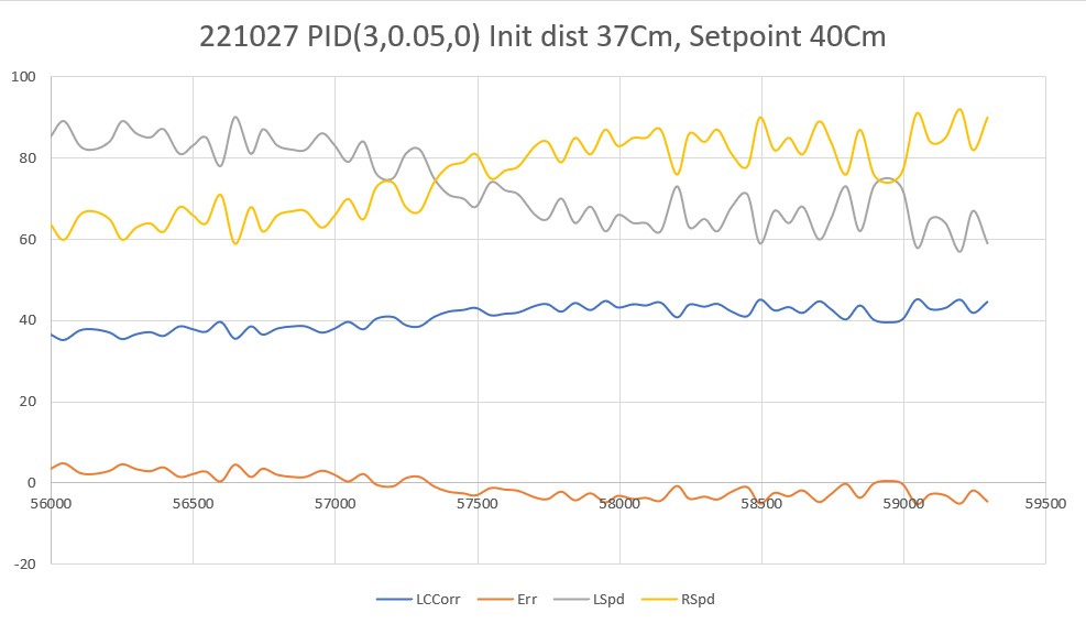
TrackRightWallOffset: Start tracking offset of 40.00cm with Kp/Ki/Kd = 300.00 0.00 10.00
Msec LF LC LR RF RC RR F Fvar R Rvar Steer Set Output LSpd RSpd
77927 728 794 816 42 41 41 116 10841 49 56047 0.08 -0.01 -26.10 101 48
78023 728 794 816 43 41 42 116 10846 46 56107 0.10 -0.01 -32.80 107 42
78126 728 794 816 42 41 45 119 10845 53 56159 -0.26 -0.01 71.40 3 127
78224 728 794 816 42 41 44 117 10841 58 56198 -0.21 -0.01 60.50 14 127
78326 728 794 816 39 39 38 109 10841 54 56270 0.11 0.01 -27.00 102 48
78427 728 794 816 38 36 37 101 10844 56 56357 0.08 0.04 -12.60 87 62
78525 728 794 816 37 35 36 96 10850 65 56427 0.12 0.05 -20.70 95 54
78623 728 794 816 36 36 34 91 10852 72 56493 0.21 0.04 -50.00 125 25
78726 728 794 816 35 35 35 87 10848 71 56543 0.01 0.05 9.90 65 84
78828 728 794 816 35 34 36 84 10841 78 56607 -0.13 0.06 55.50 19 127
78927 728 794 816 34 33 34 80 10836 90 47712 -0.07 0.07 42.50 32 117
79025 728 794 816 33 31 33 74 10836 94 47751 0.04 0.09 15.90 59 90
79124 728 794 816 32 31 31 71 10836 85 40235 0.04 0.09 15.00 60 90
79223 728 794 816 32 31 32 66 10839 103 40236 -0.03 0.09 35.30 39 110
79324 728 794 816 30 29 29 61 10845 110 30500 0.11 0.11 1.20 73 76
79424 728 794 816 30 30 29 56 10855 102 30502 0.18 0.10 -23.20 98 51
79523 728 794 816 31 30 29 50 10862 108 30502 0.27 0.10 -50.10 125 24
79625 728 794 816 31 30 29 43 10877 126 30505 0.21 0.10 -33.60 108 41
79725 728 794 816 31 30 29 38 10884 126 30344 0.18 0.10 -24.30 99 50
In HandleAnomalousConditions with WALL_OFFSET_DIST_AHEAD error code detected
WALL_OFFSET_DIST_AHEAD case detected with tracking case Neither
In SpinTurn(CCW, 90.00, 45.00)
80675: glLeftCenterCm = 794 glRightCenterCm = 24
glLeftCenterCm > glRightCenterCm --> Calling TrackRightWallOffset()
80680: TrackRightWallOffset(), glRightFrontCm = 25
In TrackRightWallOffset with Kp/Ki/Kd = 300.00 0.00 10.00
In TrackRightWallOffset with RR/RC/RF = 25 24 25
straight window = 8 cm
R/C/F dists = 25 24 25 Steerval = 0.050, WallAngle = 2.86, Inside
In SpinTurn(CCW, 27.14, 45.00)
R/C/F dists = 25 26 28 Steerval = 0.300, WallOrientDeg = 17.14
approach start: orient angle = 17.143, tgt_distCm = 40
At start - err = prev_err = -12
R/C/F dists = 25 26 28 Steerval = 0.300, OrientDeg = 17.14, err/prev_err = -12
R/C/F dists = 25 26 28 Steerval = 0.300, OrientDeg = 17.14, err/prev_err = -12
Msec RFront RCtr RRear Orient Front Rear Err P_err
81023: Error in GetFrontDistCm() - 0 replaced with 85
81031: Error in GetFrontDistCm() - 0 replaced with 85
81035 28 27 24 24.0 85 31 -13 -12
81151 32 32 27 31.4 205 40 -8 -13
81265 35 33 29 34.3 201 45 -7 -8
81378 38 36 31 38.3 196 49 -4 -7
81496 42 38 35 32.0 191 50 -2 -4
81611 45 44 38 17.7 189 55 2 -2
At end of offset capture - prev_res*res = -4
correct back to parallel (Right side): RF/RC/RR/Orient = 45 44 38 17.71
In SpinTurn(CW, 17.71, 30.00)
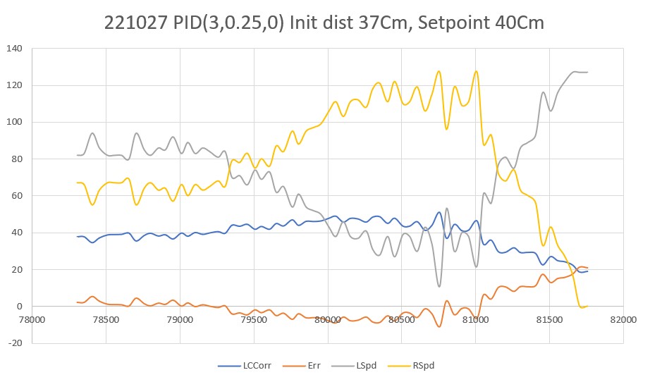
TrackRightWallOffset: Start tracking offset of 40.00cm with Kp/Ki/Kd = 300.00 0.00 10.00
Msec LF LC LR RF RC RR F Fvar R Rvar Steer Set Output LSpd RSpd
82121 113 117 126 44 46 42 134 11189 51 30097 0.19 -0.06 -72.50 127 2
82221 109 111 127 46 45 43 129 11171 57 30079 0.25 -0.05 -89.50 127 0
82321 106 110 119 45 44 43 127 11143 58 30075 0.20 -0.04 -72.60 127 2
82419 108 111 115 46 46 47 127 11105 55 30075 -0.07 -0.06 0.50 74 75
82522 728 114 120 50 49 49 128 11055 61 30081 0.02 -0.09 -31.80 106 43
82621 112 116 816 50 47 50 109 11015 71 30077 -0.03 -0.07 -12.70 87 62
82721 728 794 816 48 46 52 104 10975 69 30073 -0.32 -0.06 75.00 0 127
82820 728 794 126 44 44 46 101 10930 73 30072 -0.18 -0.04 43.20 31 118
82919 728 794 816 43 42 43 110 10854 83 30074 0.05 -0.02 -18.90 93 56
83024 728 121 816 38 37 41 264 11010 82 30086 -0.29 0.03 92.10 0 127
83124 728 794 816 35 35 37 263 11116 83 30090 -0.18 0.05 69.90 5 127
83222 728 794 816 32 32 32 163 10944 85 30098 0.01 0.08 22.60 52 97
83319 728 794 816 30 30 32 87 10840 97 30103 -0.14 0.10 70.30 4 127
83421 728 794 128 30 29 30 82 10725 101 30106 -0.01 0.11 37.20 37 112
83520 728 124 816 29 27 27 81 10581 99 30110 0.18 0.13 -13.30 88 61
83621 728 122 816 28 27 28 77 10425 102 30115 -0.04 0.13 48.80 26 123
83720 728 123 816 28 27 26 73 10555 117 30114 0.17 0.13 -9.90 84 65
83819 728 117 816 28 28 28 68 10656 108 30115 0.05 0.12 19.90 55 94
83919 728 120 816 30 29 28 66 10746 750 30115 0.29 0.11 -51.50 126 23
84018 114 123 816 31 29 27 63 10839 819 30115 0.36 0.11 -74.30 127 0
84119 112 120 816 31 30 28 57 10950 819 30115 0.29 0.10 -57.60 127 17
84217 112 118 126 31 30 30 51 11065 750 37818 0.10 0.10 -1.90 76 73
84317 728 794 816 31 30 31 45 11196 750 45125 0.00 0.10 29.00 46 104
84418 728 122 127 31 29 29 39 11339 819 53775 0.18 0.11 -19.30 94 55