Posted 03 July 2017
With this post, I’m nearing a new Personal Record for a subject series (the ‘Charging Station Design’ series went to 14), with no end in sight. The last missive from my friend and mentor John Jenkins (I’m reconsidering the ‘friend’ part, as ASFAICT, he intends to drive me into an early grave over this project!) was ‘Still not there – the ‘Final Value’ output from the filter is still wrong! :-(.
Be that as it may, it is my lot, challenge, ‘opportunity to excel’ or whatever, to continue working on this thing until I kill it – or it kills me (indeterminate as to which at the moment) 😉
So, after eliminating most/all of the print statements, John is still convinced that the Teensy is missing samples on a regular basis, and this is screwing up the rest of the algorithm. I’m just as convinced that the Teensy is way too fast to miss any samples, and that any problems must be later in the algorithm.
However, there may be a way to settle which is which, without the use of magic or a crystal ball. The Teensy 3.5/3.6 SBC’s come with a built-in micro-SD card capability, which I think can be used to log the output of each stage in a way that doesn’t (I hope) impact sample timing.
The first step in my new master plan is to make sure I can actually write to and read from an SD card on my demod Teensy (actually my first step was to go by MicroCenter and get a micro-SD card, as all mine seem to have disappeared!). I found and loaded PaulStoffregen Paul Stoffregen’s nice little SD test sketch from his GitHub site, and ran it on my Teensy 3.5. After changing the ‘chipSelect’ constant from the default 4 to ‘BUILTIN_SDCARD’, it ran successfully, and I was even able to open the ‘Test.txt’ on my PC – Yay!
The next step is to modify my IR demod program to send logging data to the SD card instead of the serial port, and to monitor my timing pulse output to make sure the SD card writes don’t interfere (can’t imagine they would, but I have a very limited imagination!).
After timing a loop that wrote 1000 short lines to the SD card, I reluctantly came to the conclusion that the stock SD card library may not be fast enough to ensure that logging output isn’t affecting the results of the algorithm. There is a faster library (SdFat), and some other speedup techniques, but rather than going down yet another rabbit-hole, I decided it was time to try a different idea.
The original plan for the IR demod idea was to use a ~520Hz square-wave modulation frequency. This is high enough to be well away from 60Hz line freq, and not aligned with higher line harmonics, but it may be just high enough to be causing the problems we are seeing. Since the algorithm actually doesn’t care what the frequency is, I decided that I can put the timing issue to bed by simply reducing the modulation frequency by a factor of 10, to something like 52Hz. Sample spacing at this frequency (assuming 20 samples/cycle) is 1000μS, which should provide more than enough room for computations (and hopefully some printouts).
To start this process, I modified both the transmit and receive Teensy 3.5 programs for the new, lower freq, and then tweaked the transmit frequency to synch with the receiver timing. As the following short video shows, a transmit frequency of 51.87Hz and a receive frequency of 51.815Hz synched up fairly well.
The demodulator timing pulse train (the rising edge is at the start of the sampling/computation block,and the trailing edge is at the end) is shown in the following scope photos.
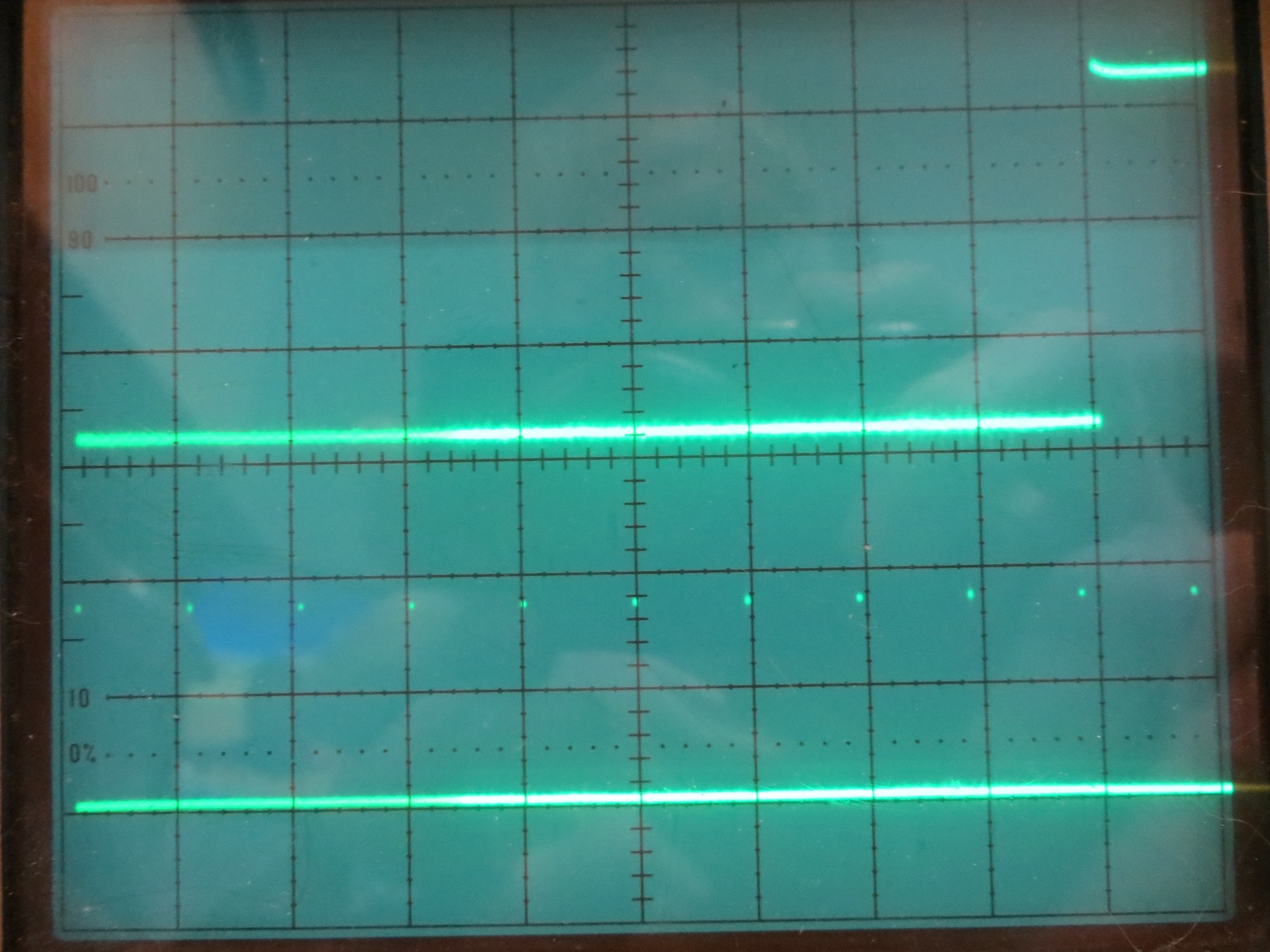
Bottom trace is sampler pulse train, top trace is square wave at ~52Hz. Time scale is 1ms/cm
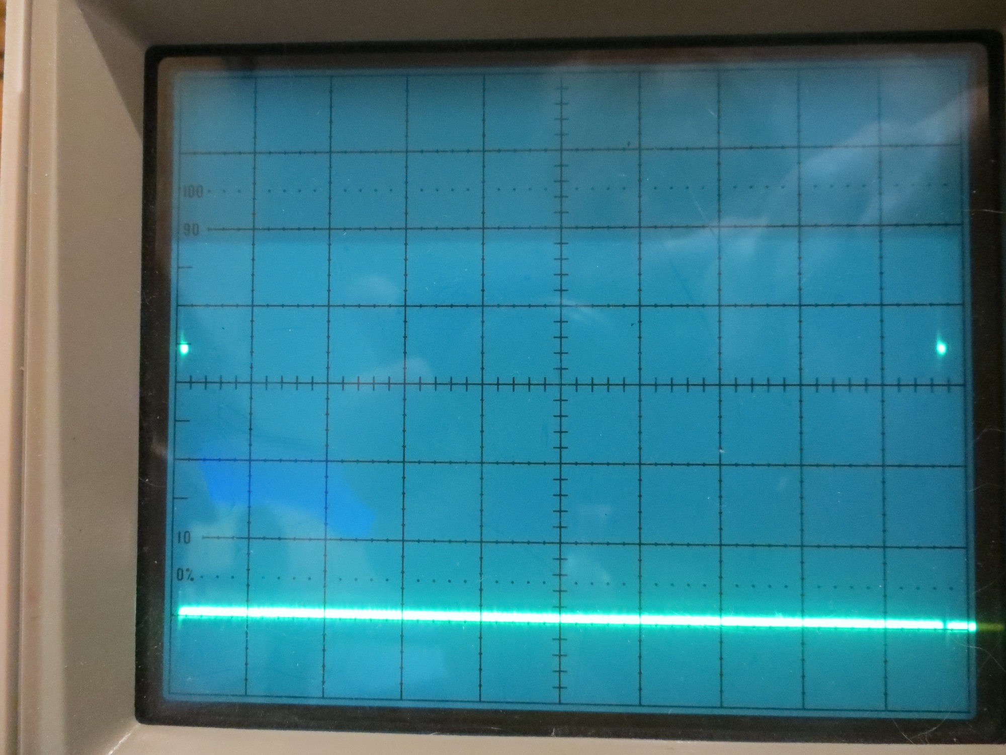
Photo showing just one sampling period. Time scale is 0.1ms/cm
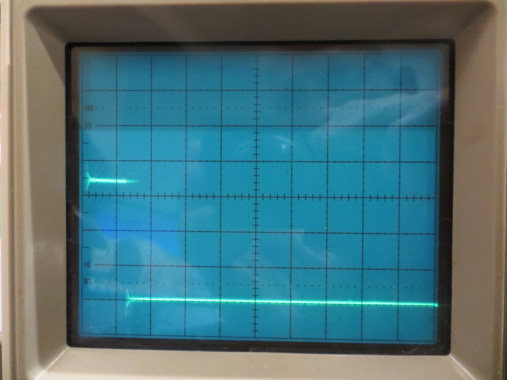
Expanded view of one sampling/computation period. Time scale is 5 microsec/cm
From the above photos, it is clear that the entire sampling/computation block takes less than 10μS, leaving about 990μS free before the next sample occurs.
Yesterday, ‘talking’ about this problem (‘talking’ with John can be a rather terrifying experience – sort of like ‘talking’ with Zeus – you wonder when the thunderbolt will arrive and whether or not he’s going to miss) with John, I opined that if his theory of missing samples is correct, a list of accurate sample timestamps should show some gaps; a linearly increasing timestamp value would refute the claim, and a plot with vertical jumps would validate it.
Then last night, as I was drifting off to sleep, I realized I didn’t have to actually create the necessary timestamps, as I already had them in the code. The elapsedMicros variable type such as ‘sinceLastSample’ gets incremented by the system each time through loop(), and only gets modified from inside the sampling/computation loop. If all samples are taken on time, this variable should be a constant when measured inside the sample/computation block just before it gets reset. The relevant code snippet is shown below
|
1 2 3 4 5 6 7 |
//this runs every 95.7uSec if (sinceLastSample > USEC_PER_SAMPLE) { /*RECORD sinceLastSample HERE!*/ //sinceLastSample = 0; sinceLastSample -= USEC_PER_SAMPLE; |
At the point shown by “/*RECORD sinceLastSample HERE!*/” in the above snippet, the ‘sinceLastSample’ variable should be USEC_PER_SAMPLE +/- 1μS. A dropped sample event should cause the value of this variable to change to N*USEC_PER_SAMPLE, where N is the number of consecutive dropped samples.
So, all I have to do is write the ‘sinceLastSample’ value to an array for a few seconds, and then write it back out again after stopping the program. An Excel plot of the values should tell the tale, one way or the other
05 July 2017
Here are some preliminary results from the 52Hz implementation
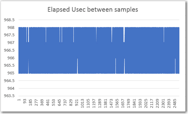
A 2560-point (128 cycles) array containing ‘sinceLastSample’ values.
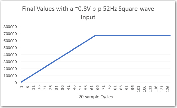
129-point array containing ‘Final Value’ values
Note that the ‘sinceLastSample’ value varies -0/+3 μS from ideal (the actual value is something like 964.32 μS), and there are clearly no dropped samples.
The ‘Final Value’ curve looks rather linear up to something like 680,000, which I suspect John is going to confirm is the correct value for a 0.8V p-p squarewave input at the center freq of the filter passband.
So, assuming John does indeed confirm the final value numbers are correct, pretty much validates the algorithm (unchanged from the 520Hz version), and lends credence to his idea that samples are getting dropped in the higher frequency implementation.
More to come,
Frank
Pingback: IR Modulation Processing Algorithm Development – Part XIV - Paynter's Palace