Posted 24 June 2017
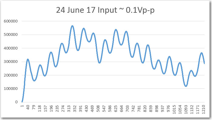
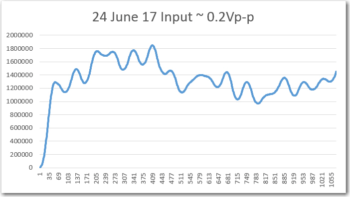
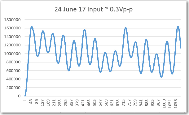
Well, I may have spoken too soon about the perfection of my implementation of John’s ‘N-path’ band-pass filter (BPF) intended to make Wall-E2 impervious to IR interference. After my last post on this subject, I re-ran some of the ‘Final Value’ plots for different received IR modulation amplitudes and the results were, to put it bluntly, crap 🙁 . Shown below is my original plot from yesterday, followed by the same plot for different input amplitudes
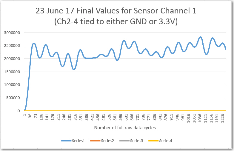
Computed final values vs complete input data cycles for sensor channel 1 (This is the original from yesterday)
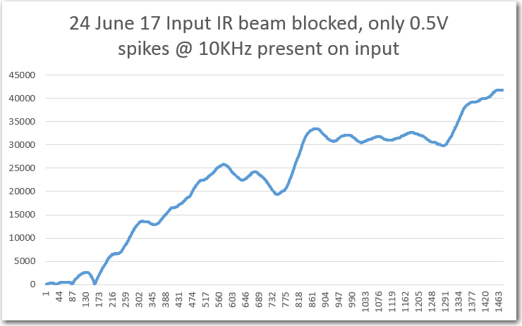
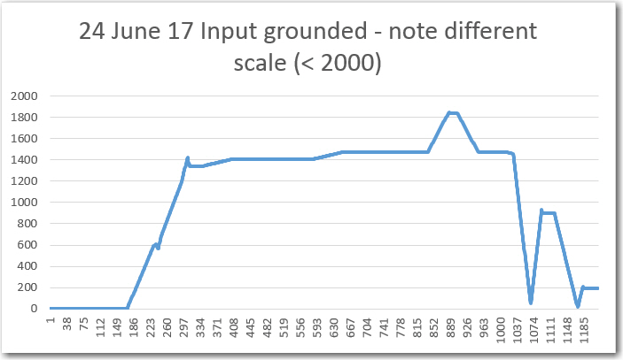
So, clearly something is ‘fishy in Denmark’ here, when the ‘no-signal’ case with only high-frequency noise causes the output to increase without limit, and the ‘input grounded’ case is decidedly non-zero (although the values are much lower than in the ‘signal present’ cases).
Time to go back through the entire algorithm (again!) looking for the problem(s).
25 June 2017
My original implementation of the algorithm was set up to handle four sensor input channels, so each step of the process required an iteration step to go through all four, something like the code snippet below:
|
1 2 3 4 5 6 7 8 9 |
//Step1: Collect a 1/4 cycle group of samples for each channel and sum them into a single value // this section executes each USEC_PER_SAMPLE period for (int i = 0; i < NUMSENSORS; i++) { //07/20/17 rev to capture raw data for later readout int samp = adc->analogRead(aSensorPins[i]); aSampleSum[i] += samp; } SampleSumCount++; //goes from 0 to SAMPLES_PER_GROUP-1 |
In order to simplify the debug problem, I decided to eliminate all these iteration steps and just focus on one channel. To do this I ‘branched’ my project into a ‘SingleChannel’ branch using GIT and TortoiseGit’s wonderful GIT user interface (thanks TortoiseGit!). This allows me to muck about in a new sandbox without completely erasing my previous work – yay!
Anyway, I eliminated all the 4-sensor iteration steps, and went back through each step to make sure each was operating properly. When I was ‘finished’ (I never really finish with any program – I just tolerate whatever level of bugs or imperfections it has for some time). After this, I ran some tests for proper operation using just one channel. For these tests, the Teensy ADC channel being used was a) grounded, b) connected to 3.3VDC, c) unterminated. For each condition I captured the ‘Final Value’ output from the algorithm and plotted it in Excel, as shown below.
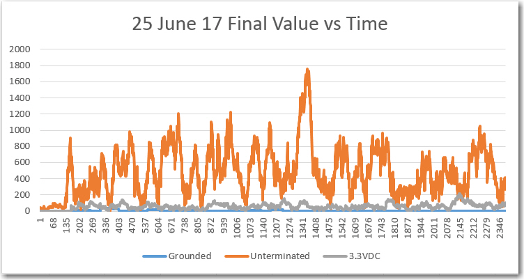
Single channel testing with grounded, unterminated, and +3.3VDC input
As can be seen from the above plot, things seem to be working now, at least for a single channel. The ‘grounded’ and ‘3.3VDC’ cases are very nearly zero for all time, as expected, and the ‘unterminated’ case is also very low.
Next, I added a 0.5V p-p signal at ~520Hz to the sensor input, and re-ran the program. After capturing the ‘Final Value’ data as before, I added it to the above plot, as shown below
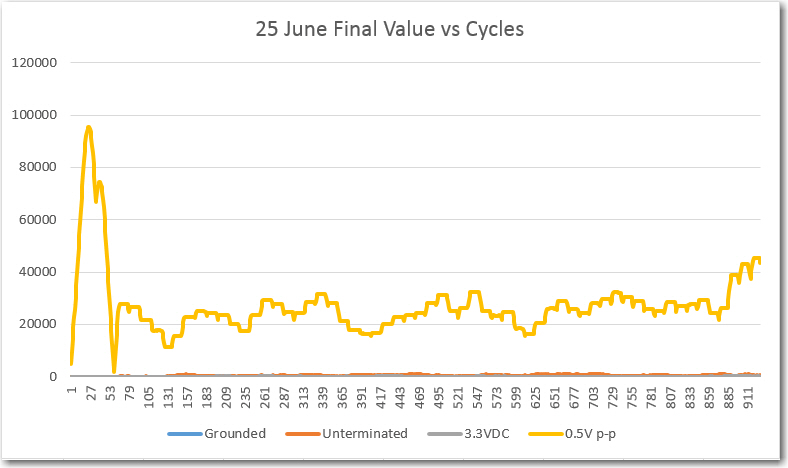
Final Value vs Cycles for 0.5V p-p input
As can be seen in the above plot, the ‘Final Value looks much more reasonable than before. When plotted on the same scale as the ‘grounded’, ‘unterminated’, and ‘+3.3VDC’ conditions, it is clear that the 0.5V p-p case is a real signal.
Then I ran a much longer term (11,820 cycles, or about 22-23 sec) test with 0.5V p-p input, with the following results.
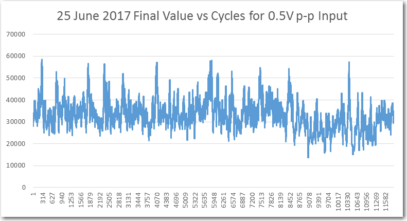
As can be seen from the above plot, the final value is a lot more ‘spiky’ than I expected. The average value appears to be around 30,000, but the peaks are more like 60,000, an approximately 3:1 ratio. With this sort of variation, I doubt that a simple thresholding operation for initial IR beam detection would have much chance of success. Hopefully, these ‘spikes’ are an artifact of one or more remaining bugs in the algorithm, and they will go away once I find & fix them 😉
Update: Noticed that there was a lot of time jitter on the received IR waveform – wonder if that is the cause of the spikes?
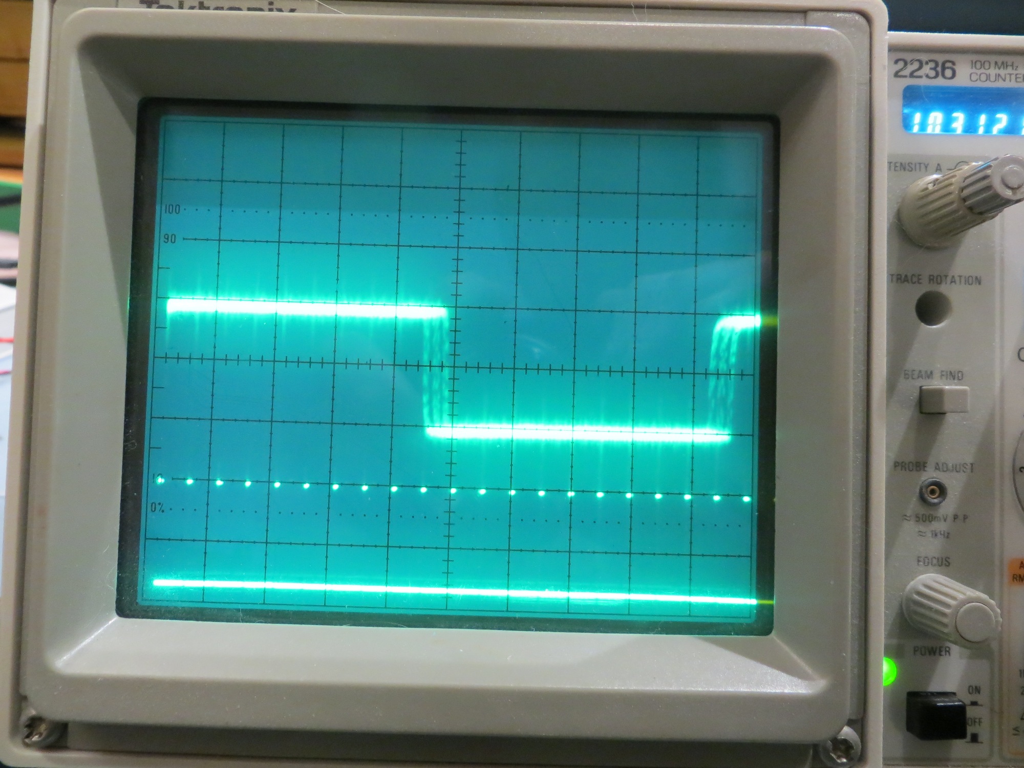
sensor waveform jitter. Note that this display is separately (Vert Mode) triggered.
Following up on this thread, I also looked at the IR LED (transmit) and photodetector (receive) waveforms together, and noted that there is quite a bit of time jitter on the Tx waveform as well, and this is received faithfully by the IR photodetector, as shown in the following short video clip
So, based on the above observations, I decided to replace the Trinket transmit waveform generator with another Teensy 3.5 to see if I could improve the stability of the transmit signal. Since I never order just one of anything, I happened to have another Teensy 3.5 hanging around, and I soon had it up and running in the setup, as shown below
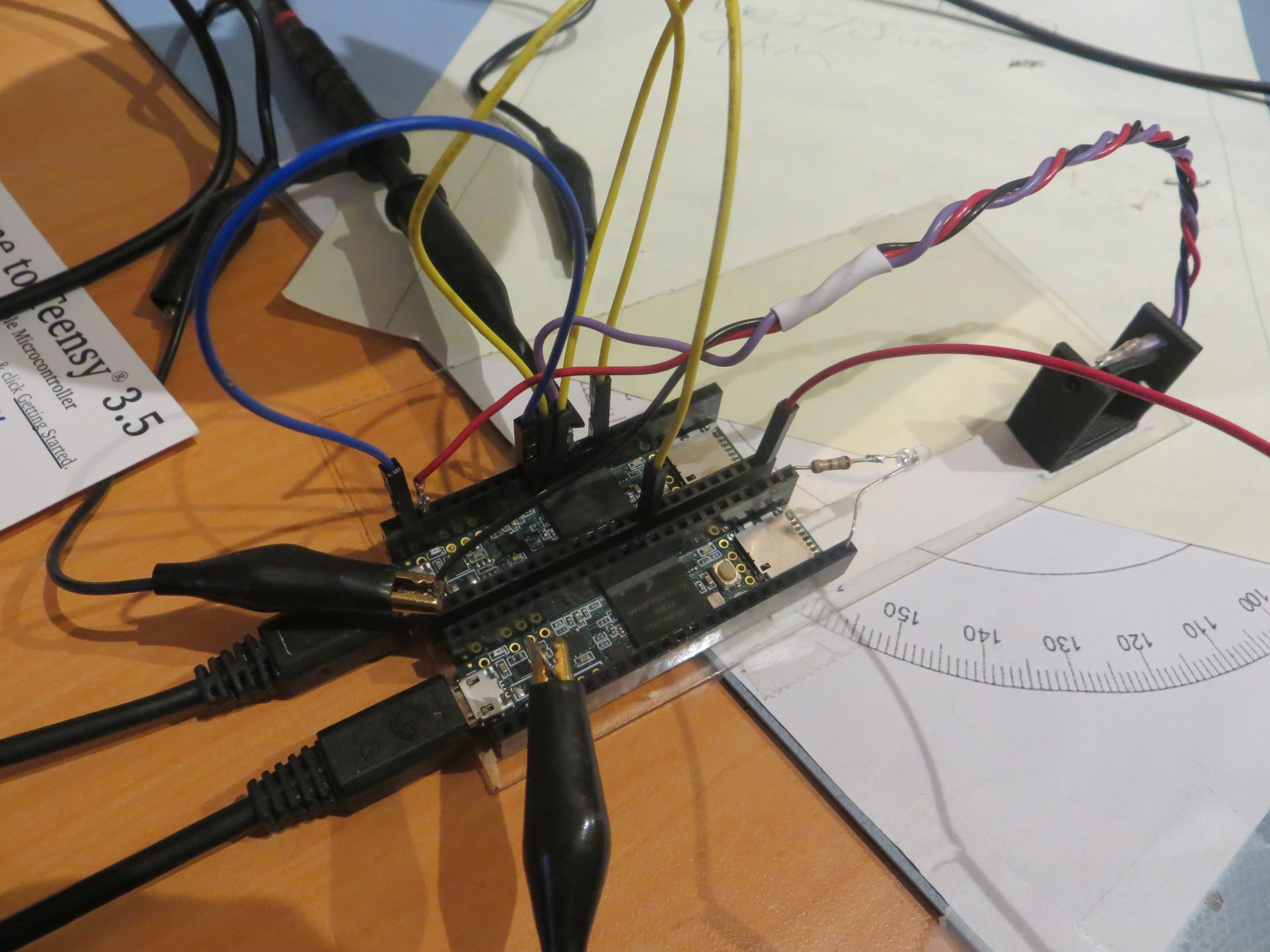
Replaced Trinket transmitter with Teensy 3.5
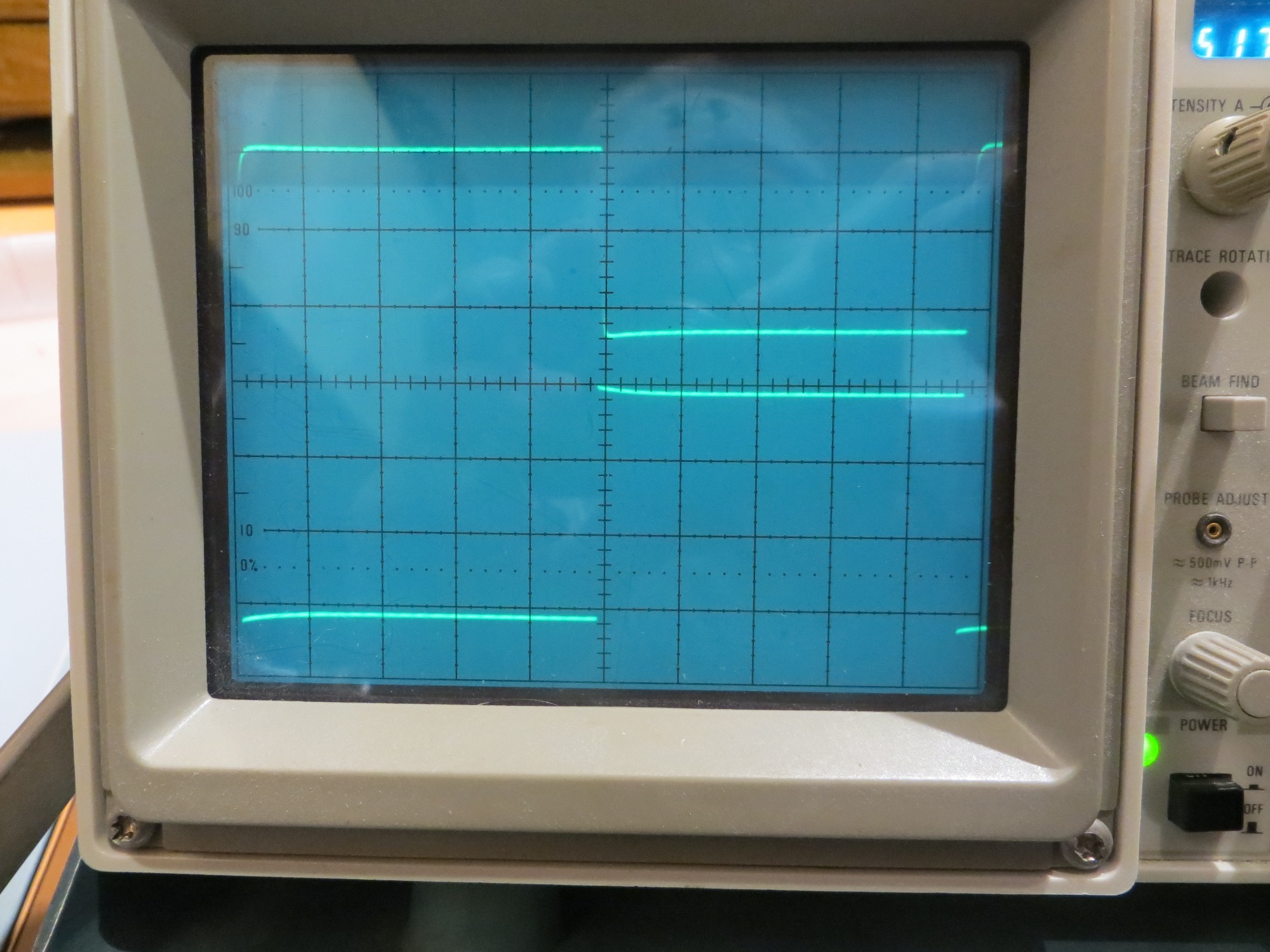
Transmit and receive waveforms
As the above short video and photos show, the Teensy implementation of the transmit waveform is much more stable than the Trinket version. Hopefully this will result in better demodulation performance.
The next step was to acquire some real data using a 0.5V p-p input signal through the IR beam path. I took this in stages, first verifying that the raw samples were an accurate copy of the input signal, and then proceeding on to the group-sum, cycle-sum, and final value stages of the algorithm.
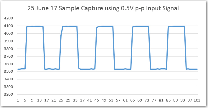
Sample capture using an input of 0.5V p-p through the IR path
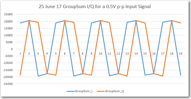
GroupSum I/Q plots using 0.5V p-p Input Signal
I then used Excel to compute the cycle sums associated with each group of 4 group sums
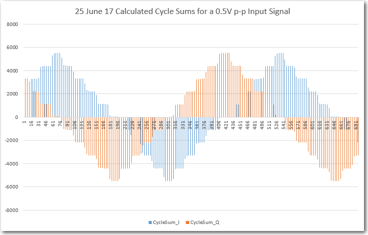
Calculated Cycle Sums for a 0.5V p-p Input Signal
And then I used Excel again to calculate the ‘Final Value’ from the previously calculated cycle sum data
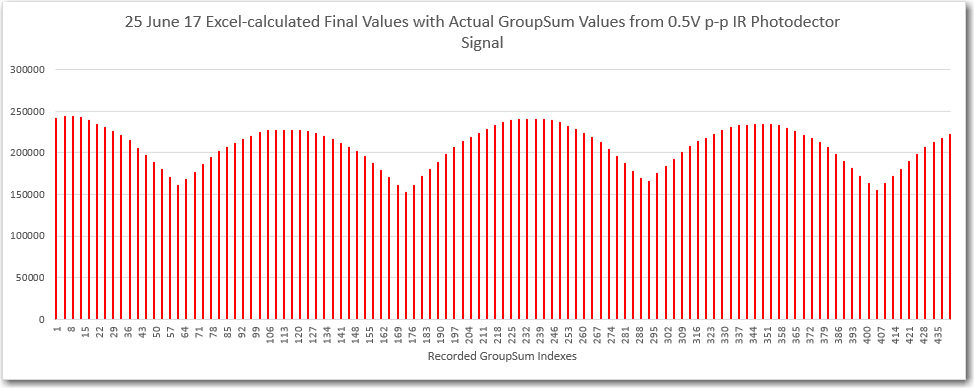
Calculated final value
Keep in mind that all the above plots are generated starting with real IR photodector data, and not that large of an input at that (0.5V p-p out of a possible 3.3V p-p).
The next step was the real ‘proof of the pudding’. I ran the algorithm again, but this time I simply printed out final values – no intermediate stages, and got the following plots
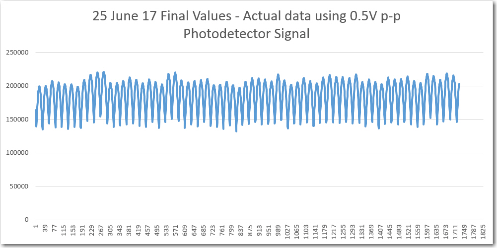
Final Value vs time, for 0.5V p-p Input Signal
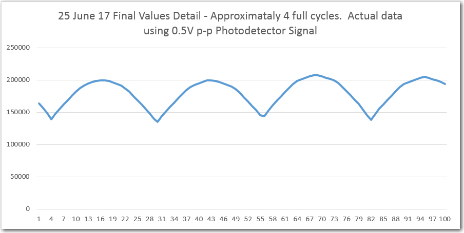
Detail of previous plot
From the above plots, I think it is clear that the algorithm is working fine, and most of the previous crappy results were caused by poor transmit timing stability. I’m not sure what causes the ripple in the above results, but I have a feeling my friend and mentor John Jenkins is about to tell me! 😉
Sleeeeeep, I need sleeeeeeeeeeep….
Frank
Pingback: IR Modulation Processing Algorithm Development – Part XV - Paynter's Palace