//Program to implement John Jenkins I/Q sq wave demod scheme
//see his sync_filter_2c.xlsx document
//Purpose (v3):
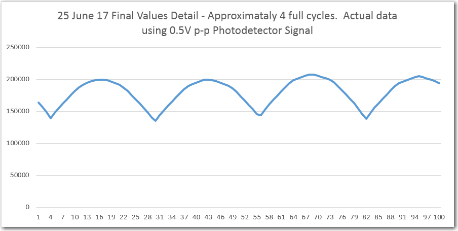
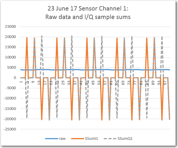
// Produce a running estimate of the magnitude of a square-wave modulated IR
// signal in the presence of ambient interferers. The estimate is computed by
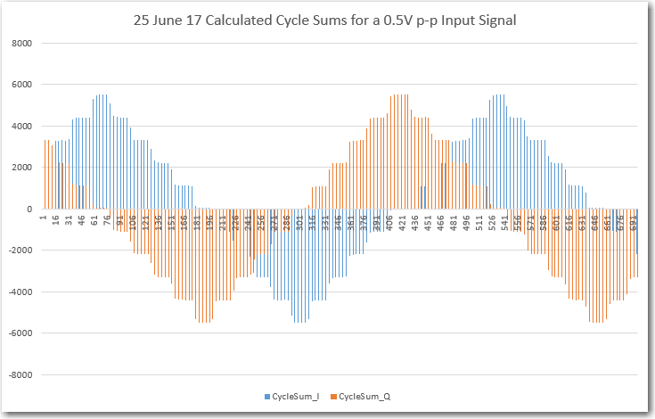
// adding the absolute values of the running sums of the I & Q outputs from a
// digital bandpass filter centered at the square-wave frequency (nominally 520Hz).
// The filter is composed of two N-element circular buffers, one for the
// I 'channel' and one for the Q 'channel'. Each element in each circular buffer
// represents one full-cycle sum of the I or Q 'channels' of the sampler. Each
// full-cycle sum is composed of four 1/4 cycle groups of samples (nominally 5
// samples/group), where each group is first summed and then multiplied by the
// appropriate sign to form the I and Q 'channels'. The output is updated once
// per input cycle, i.e. approximately once every 2000 uSec. The size of the
// nominally 64 cycle circular determines the bandwidth of the filter.
//Plan:
// Step1: Collect a 1/4 cycle group of samples and sum them into a single value
// Step2: Assign the appropriate multiplier to form I & Q channel values, and
// add the result to the current cycle sum I & Q variables respectively
// Step3: After 4 such groups have been collected and processed into full-cycle
// I & Q sums, add them to their respective N-cycle running totals
// Step4: Subtract the oldest cycle sums from their respective N-cycle totals, and
// then overwrite these values with the new ones
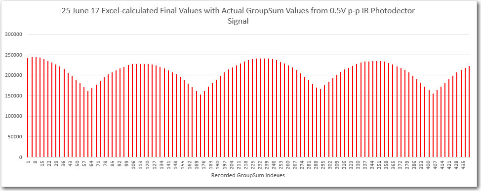
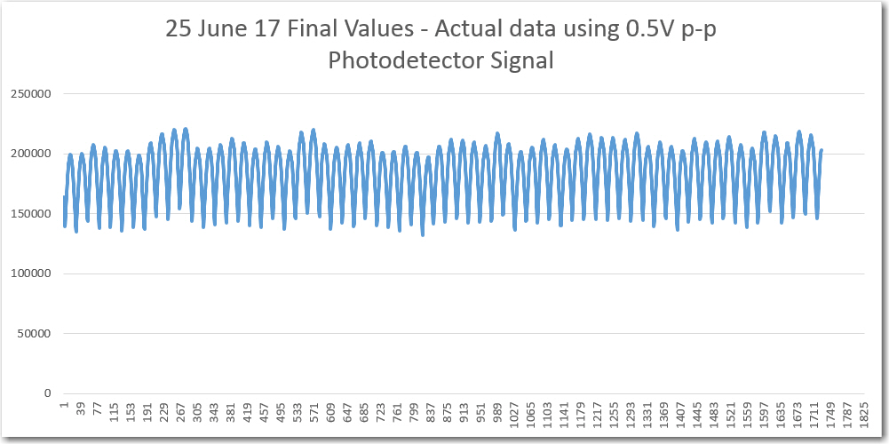
// Step5: Compute the final demodulate sensor value by summing the absolute values
// of the I & Q running sums.
// Step6: Update buffer indicies so that they point to the new 'oldest value' for
// the next cycle
//Notes:
// step 1 is done each acquisition period
// step 2 is done each SAMPLES_PER_GROUP acquisition periods
// step 3-6 are done each SAMPLES_PER_CYCLE acquisition periods
#include <ADC.h>
ADC *adc = new ADC(); // adc object;
#pragma region ProgConsts
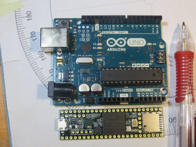
const int OUTPUT_PIN = 32; //lower left pin
const int IRDET1_PIN = A0; //aka pin 14
//const int SQWAVE_FREQ_HZ = 520; //approximate
//const int USEC_PER_SAMPLE = 1E6 / (SQWAVE_FREQ_HZ * SAMPLES_PER_CYCLE);
const int SAMPLES_PER_CYCLE = 20;
const int GROUPS_PER_CYCLE = 4;
const int SAMPLES_PER_GROUP = SAMPLES_PER_CYCLE / GROUPS_PER_CYCLE;
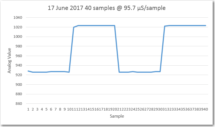
const float USEC_PER_SAMPLE = 95.7; //value that most nearly zeroes beat-note
const int RUNNING_SUM_LENGTH = 64;
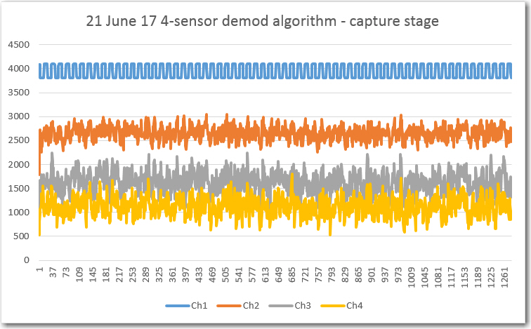
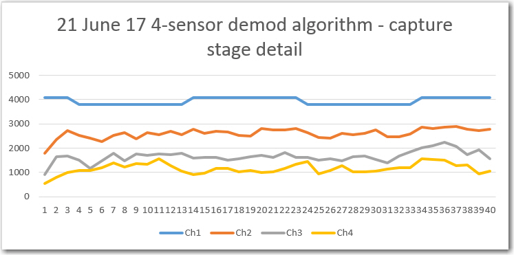
const int NUMSENSORS = 4;
const int aSensorPins[NUMSENSORS] = { A0, A1, A2, A3 };
const int aMultVal_I[GROUPS_PER_CYCLE] = { 1, 1, -1, -1 };
const int aMultVal_Q[GROUPS_PER_CYCLE] = { -1, 1, 1, -1 };
#pragma endregion Program Constants
#pragma region ProgVars
int aSampleSum[NUMSENSORS];//sample sum for each channel
int aCycleGroupSum_Q[NUMSENSORS];//cycle sum for each channel, Q component
int aCycleGroupSum_I[NUMSENSORS];//cycle sum for each channel, I component
int aCycleSum_Q[NUMSENSORS][RUNNING_SUM_LENGTH];//running cycle sums for each channel, Q component
int aCycleSum_I[NUMSENSORS][RUNNING_SUM_LENGTH];//running cycle sums for each channel, I component
int RunningSumInsertionIndex = 0;
int aRunningSum_Q[NUMSENSORS];//overall running sum for each channel, Q component
int aRunningSum_I[NUMSENSORS];//overall running sum for each channel, I component
int aFinalVal[NUMSENSORS];//final value = abs(I)+abs(Q) for each channel
#pragma endregion Program Variables
elapsedMicros sinceLastOutput;
int SampleSumCount; //sample sums taken so far. range is 0-4
int CycleGroupSumCount; //cycle group sums taken so far. range is 0-3
void setup()
{
Serial.begin(115200);
pinMode(OUTPUT_PIN, OUTPUT);
pinMode(IRDET1_PIN, INPUT);
digitalWrite(OUTPUT_PIN, LOW);
//decreases conversion time from ~15 to ~5uSec
adc->setConversionSpeed(ADC_CONVERSION_SPEED::HIGH_SPEED);
adc->setSamplingSpeed(ADC_SAMPLING_SPEED::HIGH_SPEED);
adc->setResolution(12);
adc->setAveraging(1);
}
void loop()
{
//this runs every 95.7uSec
if (sinceLastOutput > 95.7)// stopped
{
sinceLastOutput = 0;
//start of timing pulse
digitalWrite(OUTPUT_PIN, HIGH);
// Step1: Collect a 1/4 cycle group of samples for each channel and sum them into a single value
// this section executes each USEC_PER_SAMPLE period
Serial.print("SampleSumCount = "); Serial.println(SampleSumCount);
for (int i = 0; i < NUMSENSORS; i++)
{
aSampleSum[i] += adc->analogRead(aSensorPins[i]);
}
SampleSumCount++; //goes from 0 to SAMPLES_PER_GROUP-1
// Step2: Every 5th acquisition cycle, assign the appropriate multiplier to form I & Q channel values, and
// add the result to the current cycle sum I & Q variables respectively
if(SampleSumCount == SAMPLES_PER_GROUP) //an entire sample group sum is ready for further processing
{
SampleSumCount = 0; //starts a new sample group
Serial.print("CycleGroupSumCount = "); Serial.println(CycleGroupSumCount);
for (int j = 0; j < NUMSENSORS; j++)
{
aCycleGroupSum_I[j] += aSampleSum[j] * aMultVal_I[j]; //add new I comp to cycle sum
aCycleGroupSum_Q[j] += aSampleSum[j] * aMultVal_Q[j]; //add new Q comp to cycle sum
}
CycleGroupSumCount++;
}//if(SampleSumCount == SAMPLES_PER_GROUP)
// Step3: After 4 such groups have been collected and processed into full-cycle
// I & Q sums, add them to their respective N-cycle running totals
if(CycleGroupSumCount == GROUPS_PER_CYCLE) //now have a complete cycle sum for I & Q - load into running sum circ buff
{
CycleGroupSumCount = 0; //start a new cycle group next time
Serial.print("RunningSumInsertionIndex = "); Serial.println(RunningSumInsertionIndex);
for (int k = 0; k < NUMSENSORS; k++)
{
// Step4: Subtract the oldest cycle sums from their respective N-cycle totals, and
// then overwrite these values with the new ones
int oldestvalue_I = aCycleSum_I[k][RunningSumInsertionIndex];
int oldestvalue_Q = aCycleSum_Q[k][RunningSumInsertionIndex];
aRunningSum_I[k] = aRunningSum_I[k] + aCycleGroupSum_I[k] - oldestvalue_I;
aRunningSum_Q[k] = aRunningSum_Q[k] + aCycleGroupSum_Q[k] - oldestvalue_Q;
aCycleSum_I[k][RunningSumInsertionIndex] = aCycleGroupSum_I[k];
aCycleSum_Q[k][RunningSumInsertionIndex] = aCycleGroupSum_Q[k];
// Step5: Compute the final demodulate sensor value by summing the absolute values
// of the I & Q running sums
int RS_I = aRunningSum_I[k]; int RS_Q = aRunningSum_Q[k];
aFinalVal[k] = abs((int)RS_I) + abs((int)RS_Q);
}
// Step6: Update buffer indicies so that they point to the new 'oldest value' for
// the next cycle
RunningSumInsertionIndex++;
if (RunningSumInsertionIndex >= RUNNING_SUM_LENGTH) RunningSumInsertionIndex = 0;
}
//end of timing pulse
digitalWrite(OUTPUT_PIN, LOW);
}//else
}//loop