Posted 25 May 2017
One of the things I didn’t understand about the analog sample runs from my previous post was why there were so many cycles of the IR modulation signal in the capture record; I had set the algorithm up to capture only 5 cycles, and there were more than 10 in the record – what gives?
Well, after a bit of on-line sleuthing, I discovered the reason was that the A/D conversion process associated with the analogRead() function takes a LOT longer than a digitalRead() operation. This put a severe dent in my aspirations for real-time processing of the modulated IR signal, as I would have to do this for at least two, and maybe four independent signal streams, in real time – oops!
One thing I have discovered for sure in the modern internet era; if you are having a problem with something, it is a certainty (i.e. Prob = 100%) that many others in the universe have had the same problem, and most likely someone has come up with (and posted about) one or more solutions. So, I googled ‘Arduino Uno faster analogRead()’, and got the following hits:
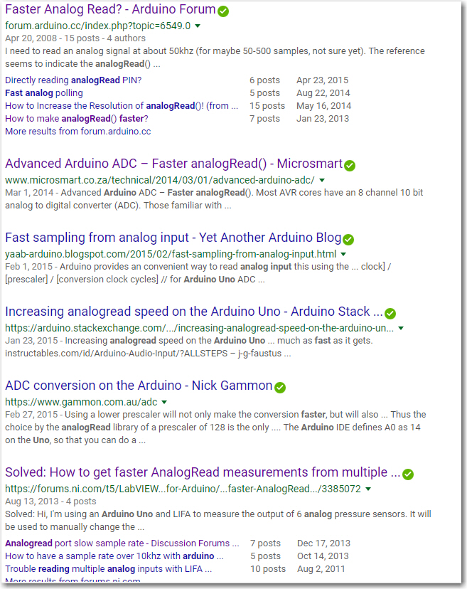
The very first link above took me to this forum post, and thanks to jmknapp and oracle, I found the Arduino code to reset the ADC clock prescale factor from 128 to 16, thereby decreasing the conversion time by a factor of 8, with no reduction in ADC resolution – neat!
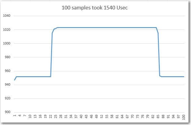
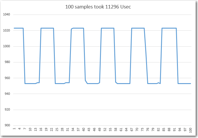
To test the effect of the prescaler adjustment, I measured the time it took for 100 ADC measurements with no delay between measurements. As shown below, there is a dramatic difference in the ‘before’ and ‘after’ plots:
100 ADC cycles with no delay, prescale = 128

100 ADC cycles with no delay, prescale = 16
Next, I adjusted the delay between ADC cycles to collect approximately 5 cycles at the 520Hz input rate, as shown below:
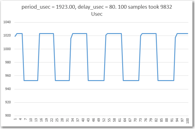
Delay adjusted so that 100 samples ~ 5 cycles at 520Hz.
With the prescaler set to 16, the ADC is much faster. With a 5-cycle collection window at 520Hz, I have 80 uSec/cycle to play with for other purposes, so it seems reasonable that I can handle multiple input streams with relative ease – YAY!!.
The next step was to simulate a 4-channel capture operation by capturing 400 samples, 100 each from four different channels. In this simulation, all the data comes from the same IR link, but the processing load and timing is the same. All the samples from the same time slot are taken within a few microseconds of each other, and the loop (inter-sample) delay was adjusted such that approximately five cycles were captured from each ‘channel’, as shown in the following Excel plot
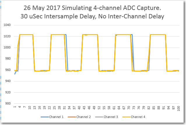
Simulated 4-channel capture
As can be seen in the above plot, the channel plots overlap almost exactly. What this shows is that the Arduino Uno can capture all four IR detector channels at sufficient time resolution (about 20 samples/cycle) for effective IR signal detection/evaluation, and with sufficient time left over (about 30 uSec) for some additional processing.
If the design is changed from four channels to just two, then the processing load goes down significantly, as shown in the following plot
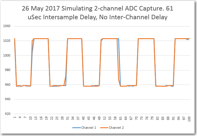
Simulated 2-channel capture
To complete the simulation, I added the code to perform the following operations on a sample-by-sample basis:
- Update the running average of the sample array
- Subtract the running average from the sample, and take the absolute value of the remainder (full-wave rectification)
- Store the result in another array so it can be plotted. This last step isn’t necessary except for debugging/evaluation purposes
Initial results as shown below are very promising. The following Excel plots show the results of processing 100 ADC samples in real time. First 100 samples were loaded into an array to represent the last 100 samples in a real-time scenario, and the running average value was initialized to the average of all these samples. Then each subsequent real-time sample was processed using the above algorithm and the results were placed in holding arrays for later printout, with the following results
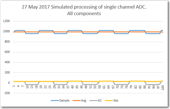
All components – original captured samples, running average, AC component, and full-wave rectified component
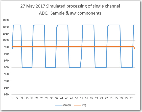
Detail view of original captured samples and the running average component
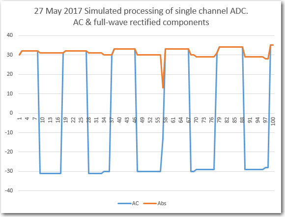
Detail view of the AC component of the original captured samples and the computed full-wave rectifed component
The above plots confirm that the ADC samples can indeed be processed to yield the full-wave rectified intensity of a modulated IR beam. However, there is a fly in the ointment – it takes too long; it took 17,384 μSec to process 100 samples – but 100 samples at 20 samples/cycle only takes approximately 9600 μSec – and this is only for one channel :-(. I will need to find some serious speedup tricks, or reduce the number of samples/cycle, or both in order to fit the processing steps into the time available.
Stay tuned,
Frank