Posted 27 May 2017
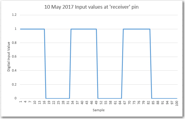
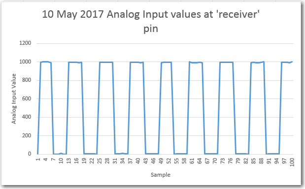
In my previous post I demonstrated an algorithm for processing a modulated IR signal to extract an intensity value, but the algorithm takes too long (at least on an Arduino Uno) to allow for 20 samples/cycle (admittedly way over the required Nyquist rate, but…). So I decided to explore ways of speeding up the algorithm.
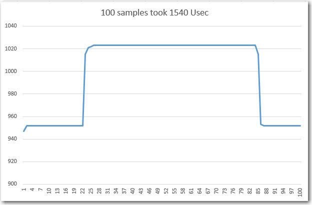
First, the baseline: The starting point is the 17,384 μSec required to process 100 samples in the current algorithm, or 174 μSec/sample. At an input frequency of 520Hz, 20 samples/cycle is about 96 μSec/sample, so I’m off by a factor of 2 or so. And this is only for one channel, so I’m really off by a factor of 4 (for a 2-channel setup) or 8 (for my current 4-channel arrangement)
As an experiment, I reduced the running average length from 5 to 1 cycles, or from 100 to 20 samples. This reduces the shifting operation load by a factor of 5, and resulted in a total processing time of 1876 μSec for all 100 samples – wow!
Then I discovered I had failed to uncomment the line that loads the new running average value into the front of the running average array, so I put that back in and re-ran the measurement. This time the number came up as 10748 μSec! This is just not possible! It is impossible that 10,000 (100 iterations/sample, 100 samples) iterations of a copy operation from one location in the array to another one takes 1/10 the time as 100 iterations (1/sample) of a copy operation from a variable into the array – not possible!!!
But, since it was happening anyway – whether possible or not, I decided I was going to have to figure it out :-(. So, I changed the line
RunningAvg1[0] = (int)chan1Avg;
to
RunningAvg1[0] = 0;
and re-ran the measurement. This time the total for processing 100 samples was 1896 μSec – much more believable! So, what’s the difference between these two operations? The only thing I could think of is that it must take a lot of time to convert a double to an int.
So, I ran a test where I executed the ‘RunningAvg1[0] = (int)chan1Avg;’ line 10 times, all by itself, and measured the elapsed time. I got 72 μSec – a much more believable number, but not what I was expecting. Increasing the number of iterations to 100 resulted in an elapsed time of 672 μSec – consistent with 72 μSec for 10 iterations. That’s nice, but I’m still not any closer to figuring out what’s going on.
Well, after a bunch more experiments, I think I have the problem narrowed down to the use of floating point math on a few operations. I have seen some posts to the effect that floating point math is much slower than integer math on Arduino processors, and these experiments tend to bear that out. I should be OK with integer math everywhere, I hope ;-).
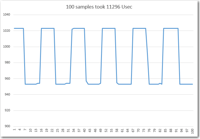
After completely re-writing the algorithm to eliminate floating point math (and correcting several logic errors – oops!), I re-ran the 100-element process for 1 channel, with the following results:
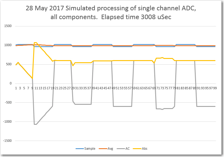
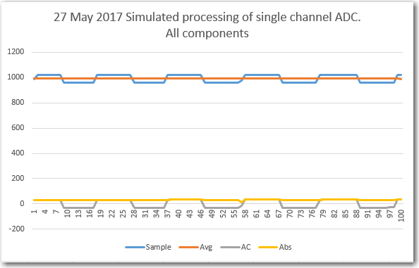
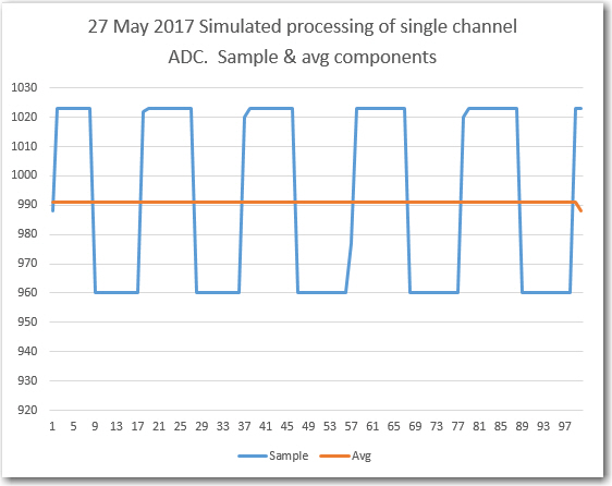
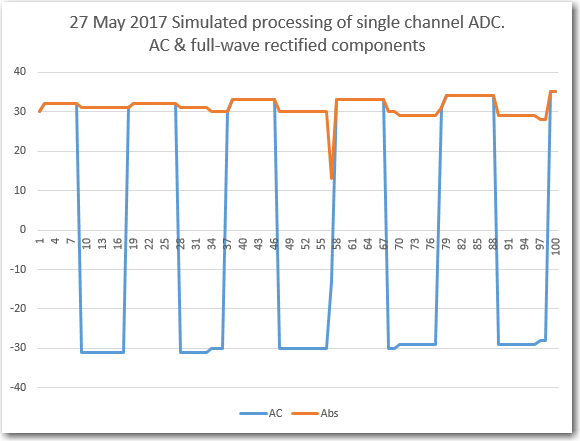
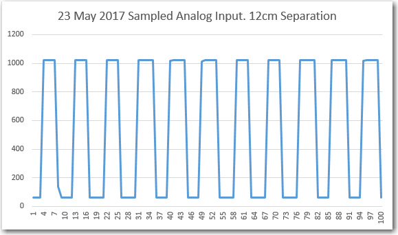
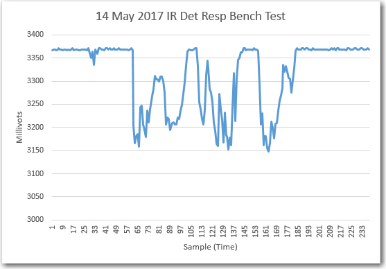
All components – original captured samples, running average, AC component, and full-wave rectified component. Note elapsed time of 3008 uSec
From the above Excel plot, it is clear that the algorithm successfully extracted the full-wave rectified value for the incoming modulated IR signal, and did so in only 3008 uSec for 100 samples. This should mean that I can easily handle up to three simultaneous channels, and maybe even four – YAY!
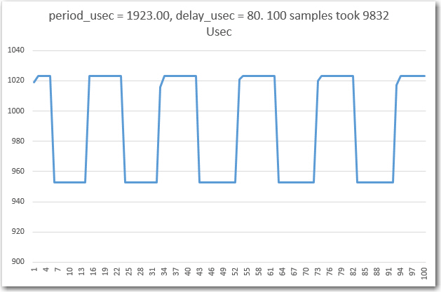
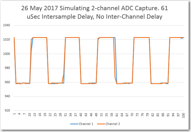
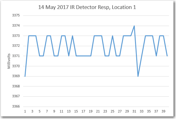
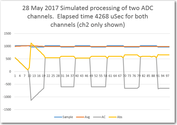
Another run with two simultaneous channels was made. The following Excel plot shows the Channel 2 results, along with the elapsed time for both channels.

Channel 2 all components – original captured samples, running average, AC component, and full-wave rectified component. Note elapsed time of 4268 uSec
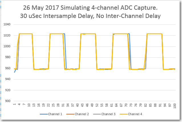
The above results for two channels strongly suggests that all four channels in the current hardware implementation can be processed simultaneously while still maintaining a 20 sample/cycle sample rate. This is extremely good news, as it implies that I can ‘simply’ insert an Arduino Uno or equivalent between the detector array and the robot controller. The robot contoller will continue to see left/right analog values as before (but inverted – more positive is more signal), but background IR interference will be averaged out by the intermediate processor – cool!
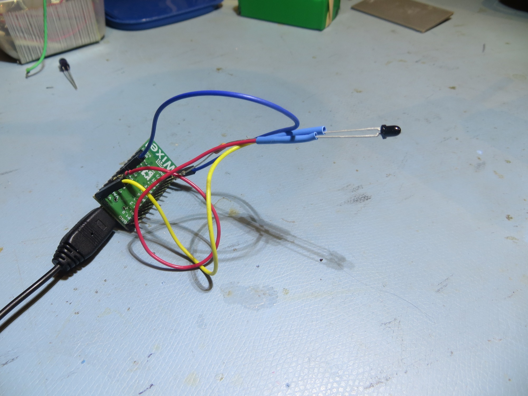
Rather than use a Uno, which is physically very large, I hope to be able to use something like an Adafruit Arduino Pro Micro, as shown below:
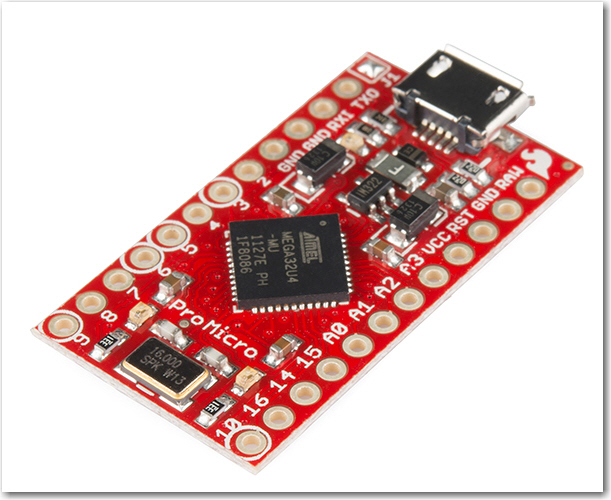
Adafruit’s Arduino Pro Micro. 16MHz, 9 Analog 12 Digital I/O
This should fit just about anywhere (probably on top of the sunshade), and be very easy to integrate into the system – we’ll see.
Stay tuned!
Frank