Monthly Archives: September 2015

End of the Road for Wall-E’s Spinning LIDAR System :-(

30 September, 2015

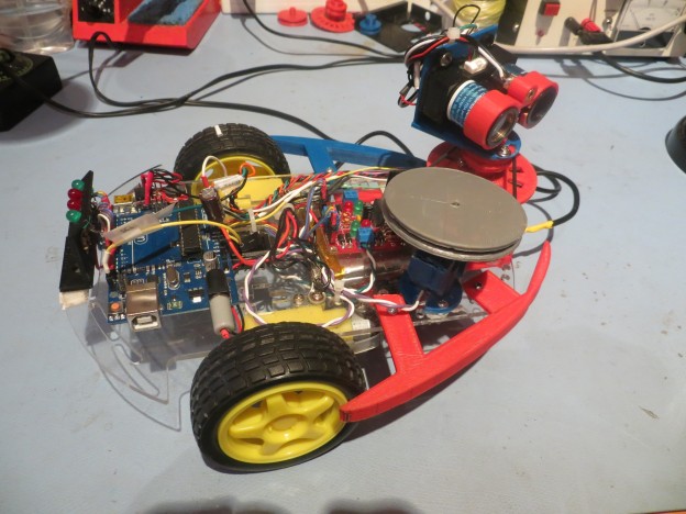
Sad to say, but I believe I have ‘hit the wall’ on development of an effective spinning-LIDAR navigation system for Wall-E.  Even with a souped-up spinning platform (approx 3 rev/sec), I have been unable to reliably navigate a straight hallway, much less recover from stuck conditions.  In addition, the combination of drive motor currents and the increased current required to drive the spinning platform at the increased rate drains  the battery in just a few minutes.  So, I have reluctantly concluded that the idea of completely replacing the acoustic sensors with a spinning-LIDAR system is a dead end; I’m going to have to go back to the original idea of using the acoustic sensors for wall following, and a fixed-orientation LIDAR for stuck detection/recovery.

I started down the spinning-LIDAR road back in April of this year, after concluding a series of tests  that proved (at least to me) that the use of multiple acoustic sensors was not going to work due to intractable multi-path and self-interference problems.  In a follow-up post at the end of that month, I speculated that I might be able to replace all the acoustic sensors  with  a spinning-LIDAR system for both wall following and ‘stuck detection’.  At the time I was aware of two good candidates for such a system – the NEATO XV-11 robot vacuum’s spinning-LIDAR subsystem, and the Pulsed Light ‘LIDAR-Lite’ component.  I chose to pursue the Pulsed-Light option because it was much smaller and lighter than the XV-11 module, and I thought it would be easier to integrate onto the existing Wall-E platform.  Part of the appeal of this option was the desire to see if I could design and build the necessary spinning platform for the LIDAR-Lite device, based on a 6-wire slipring component available through AdaFruit.

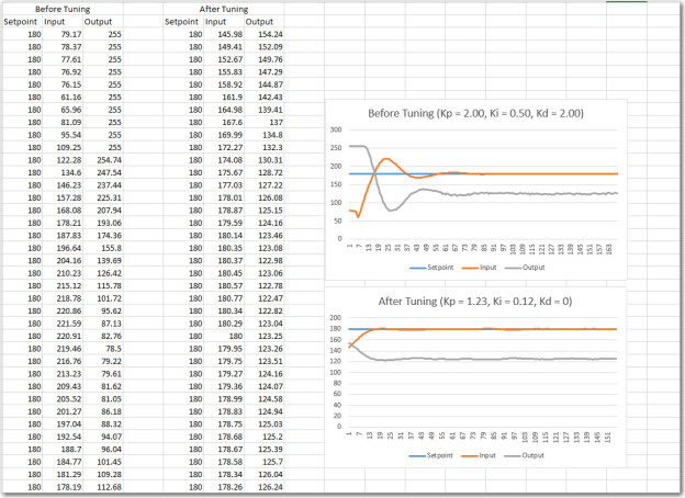
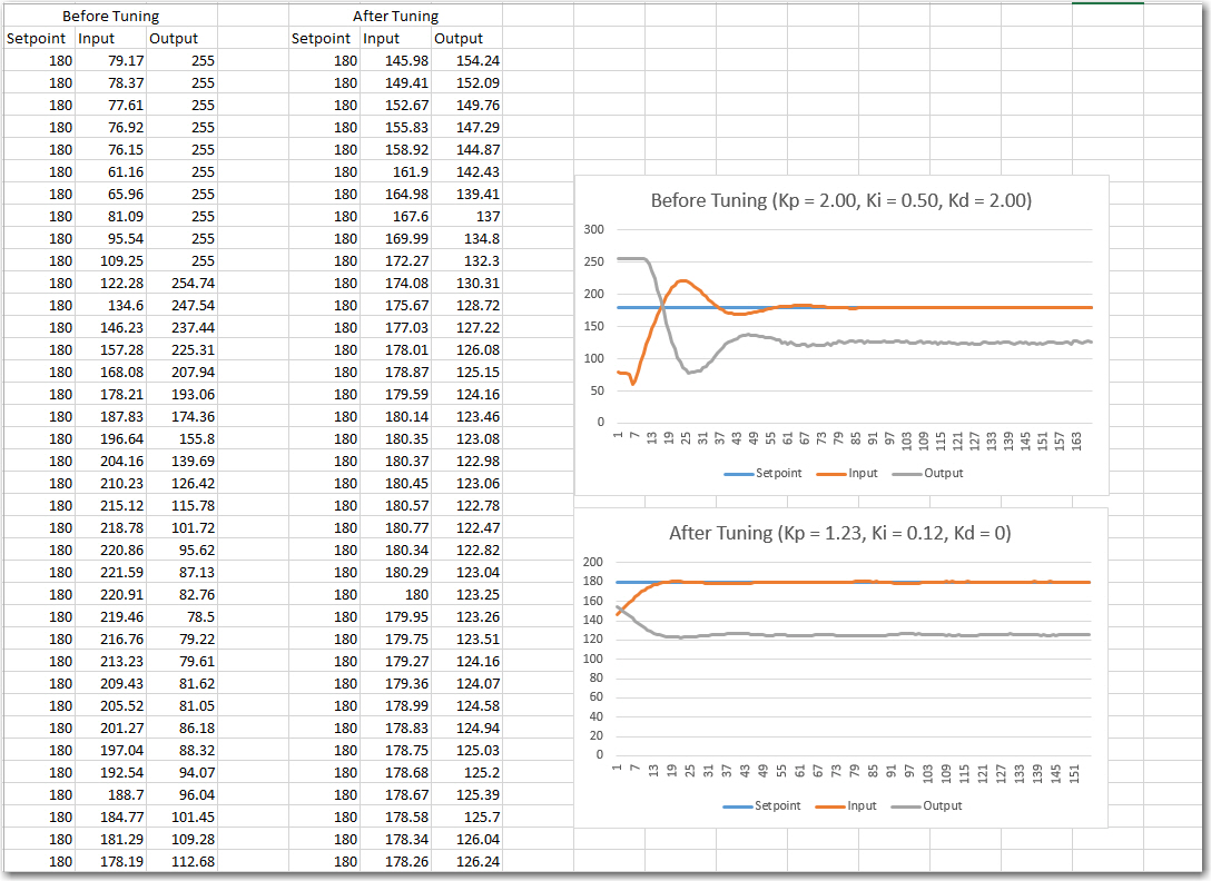
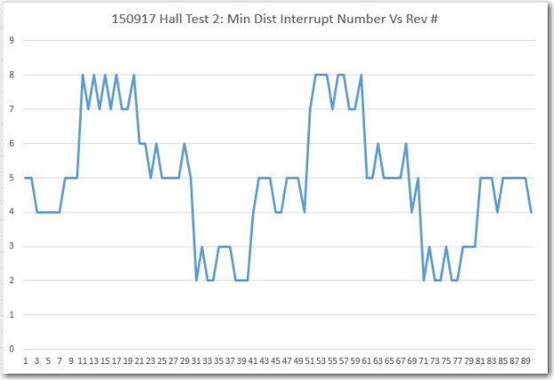
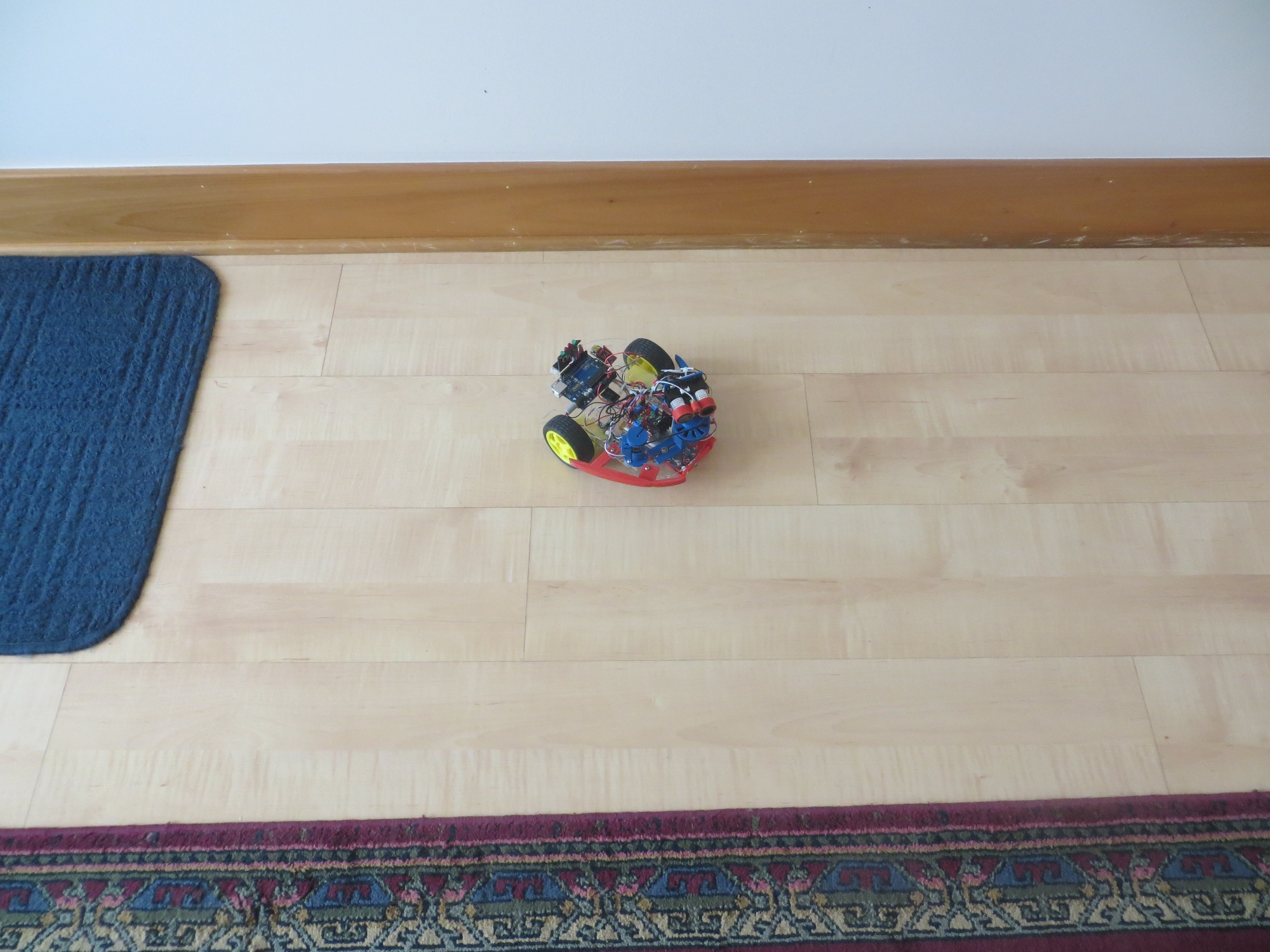
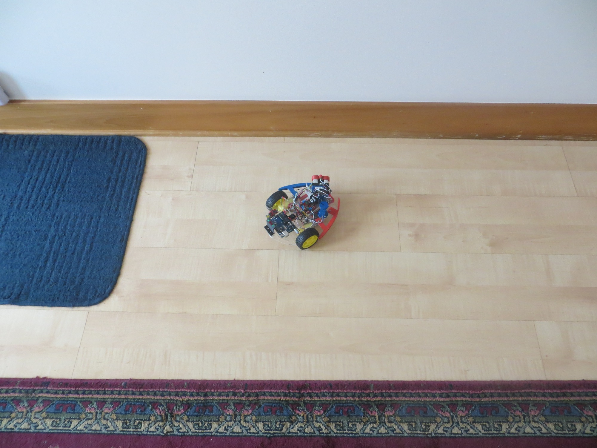
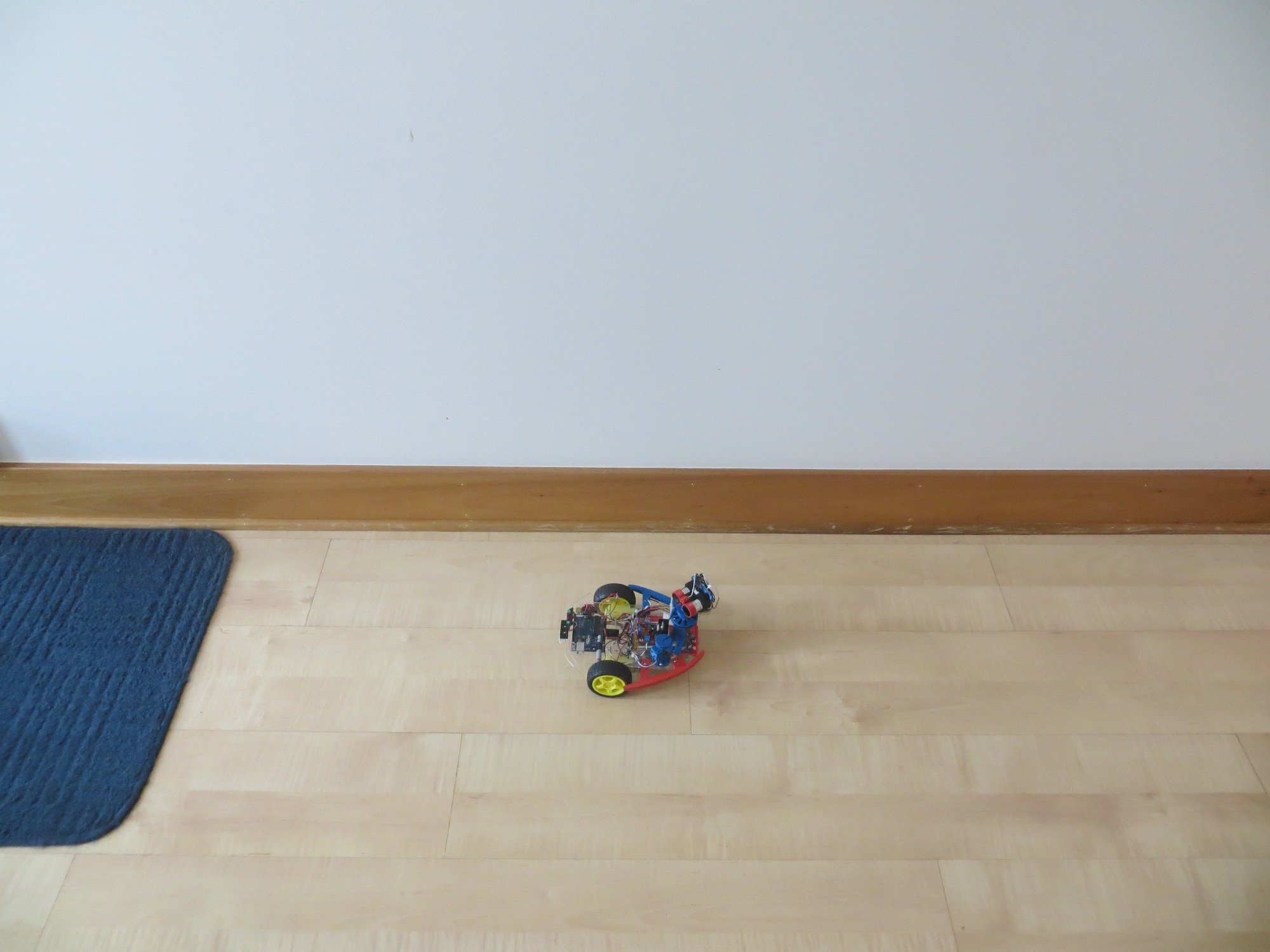
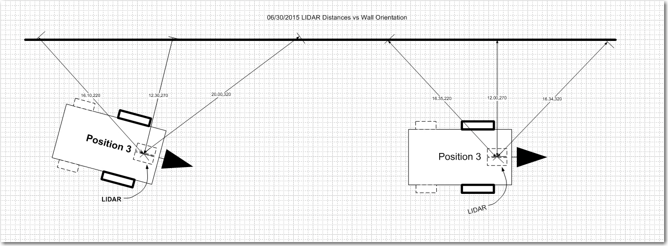
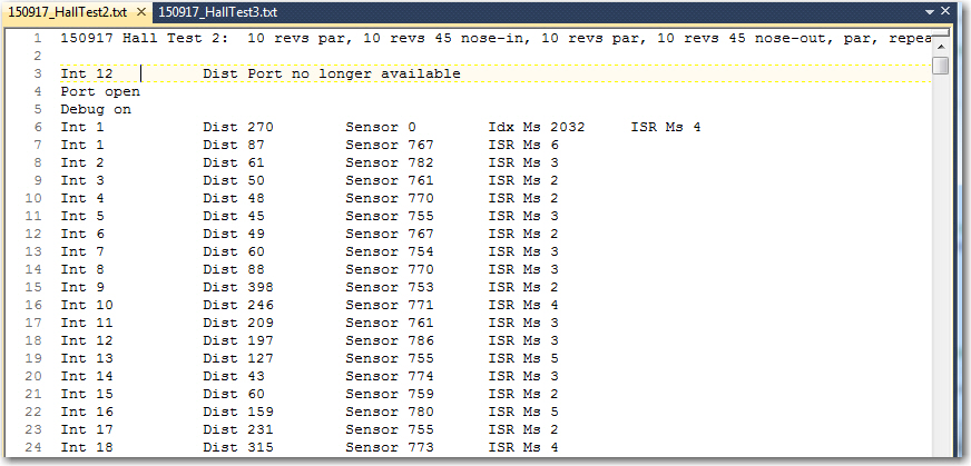
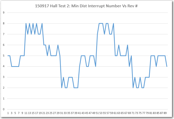
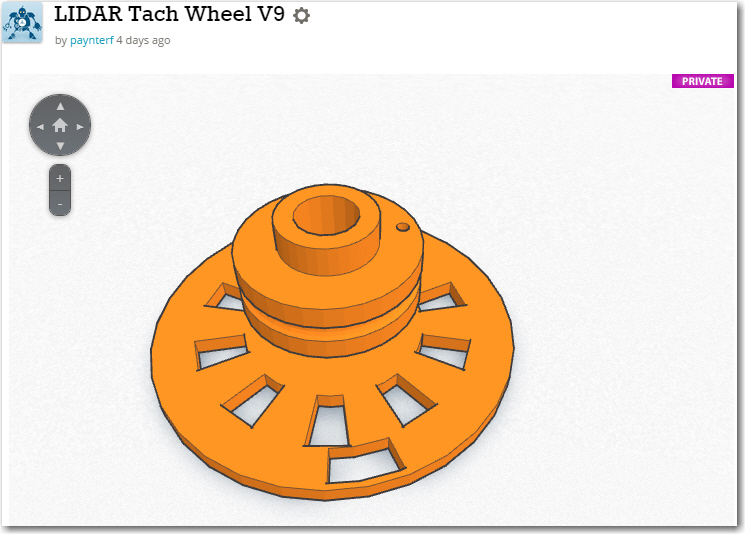
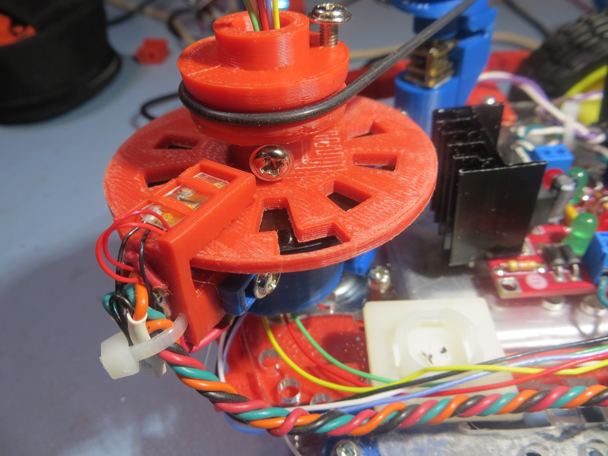
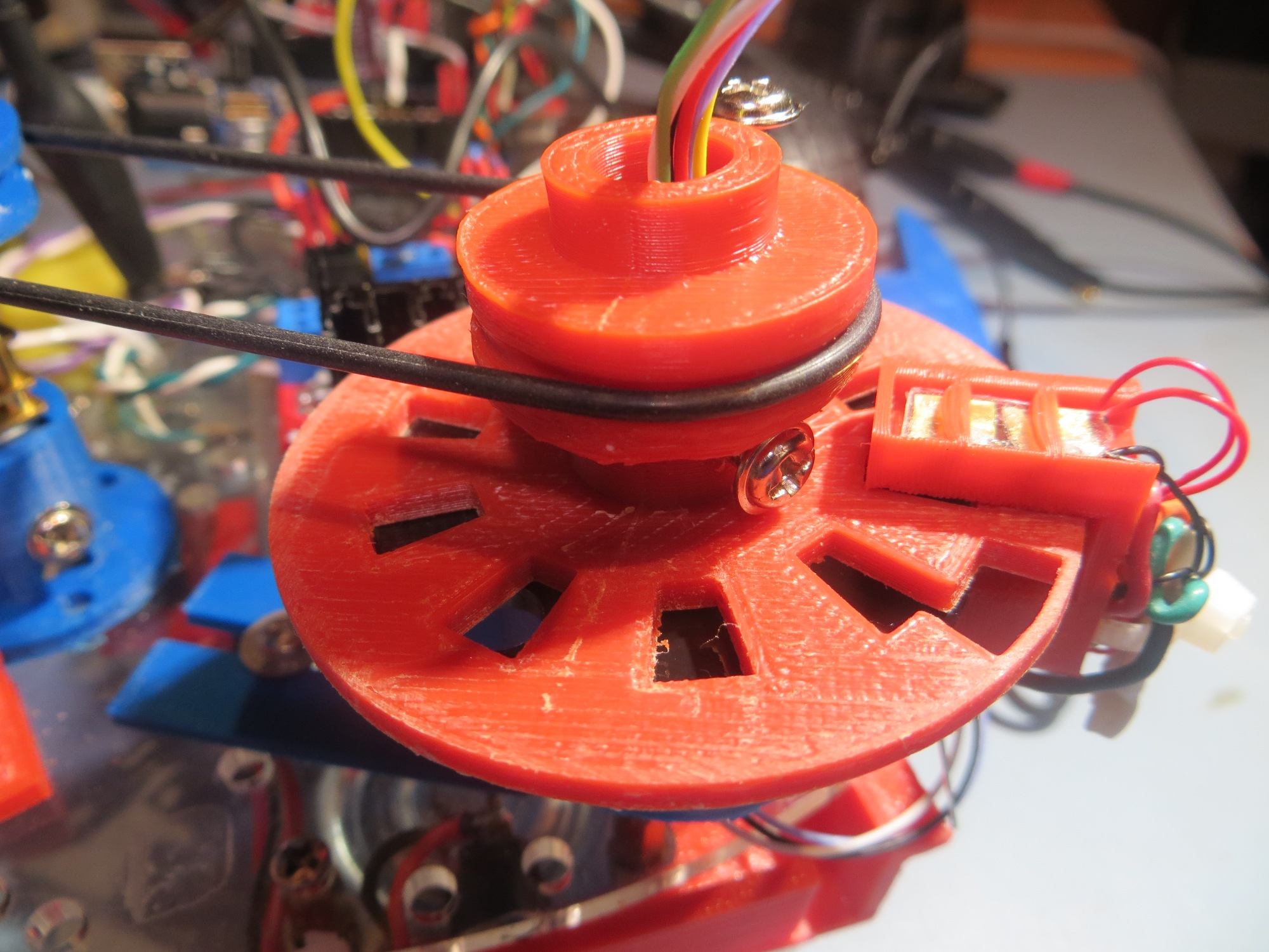
In the time since that post at the end of April, I successfully integrated the LIDAR into the Wall-E platform, but only recently got to the point of doing field tests.  The first set of tests showed me that the original spin rate of about 120 RPM (about 2 RPS) was way too slow for successful wall following using my original ‘differential min-distance’ technique, and so I spent some time investigating PID control techniques as a possibility to improve navigation.  Unfortunately, this too proved unfruitful, so I then investigated ideas for increasing the LIDAR’s spin rate.  The LIDAR spinning platform is driven by a drive belt (rubber O-ring) attached to a pulley on a separate 120 RPM DC motor.  My original setup used a pulley ratio of approximately 1:1, so the motor and LIDAR both rotated at approximately 120 RPM.  By increasing the diameter of the drive pulley, I was able to increase the LIDAR rotation rate to approximately 180 RPM (about 3 RPS), but unfortunately even that rate was too slow, and the increased drive motor current rapidly drained the batteries – rats!

'The Last Spinning LIDAR' version.  Note the large gray drive pulley.  Gets the spin rate up to around 180 RPM, but at the cost of much higher battery drain.

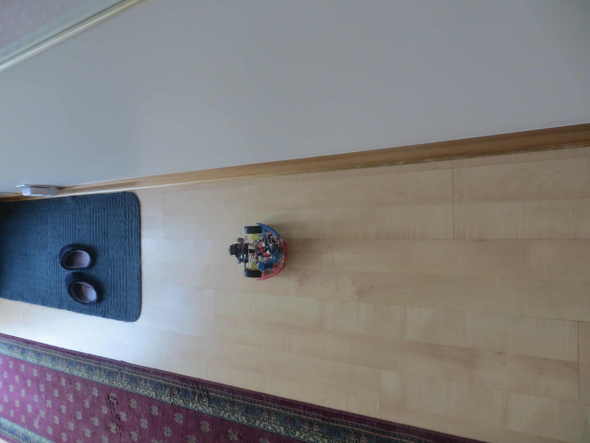
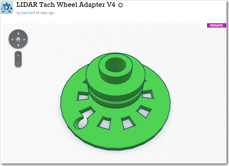
‘The Last Spinning LIDAR’ version. Note the large gray drive pulley. Gets the spin rate up to around 180 RPM, but at the cost of much higher battery drain.

So, while I had a LOT of fun, and learned a lot in the process, it’s time to say ‘Sayonara’ to the spinning-LIDAR concept (at least for Wall-E – still plan to try the XV-11 module on the 4WD robot) and go back to the idea of using acoustic sensors for wall following and a forward-looking LIDAR for obstacle avoidance and ‘stuck’ detection.

Stay tuned!

The Evolution of an Outside Shot – Part III

23 September 2015

Well, it’s been over a year since my last post on this subject, and while I’d like to say I’ve made great strides, In reality progress  has been somewhat spotty.  From November of last year  until about two months ago  I had been practicing my shot almost every day, and was seeing slow but steady improvement.  I even got to the point where I was making the occasional 3-point shot ‘in competition’ (at my age, the ‘in competition’ is  definitely in quotes!).  However, while my shooting prowess was increasing, so was pain in both my knees, and sometime in July  it got to be too much to bear anymore.  When a doctor’s visit and a set of X-rays ruled out skeletal damage as the culprit, I tried some massage therapy to see if that would help; it did, but not significantly enough to get me back on the court.  At the recommendation of the massage therapist,    I started a  physical therapy course, and although I haven’t quite finished the PT sessions, my knee pain has gone from ‘cant-stand-it-anymore’ agony to ‘mild-old-age-annoyance’ stiffness.  I’m not sure how much of this is just abstinence from shooting and how much is due to the exercises, but at this point I’m not sure I care! 😉

So, yesterday I went back to some mild practice shooting for the first time in a couple of months.  Instead of just shooting 3’s, I’m limiting my practices to short-range, foul-line, and what I call ‘2-1/2’ range (halfway between the foul line and the 3-point arc).  I was encouraged to find that the break had not erased all my skill gains (such as they were), and I was still able to shoot with a reasonable amount of good form for an ‘almost-septuagenarian’ ;-).  The following short videos show side and front views of my ‘2-1/2’ point range shooting form.   Hopefully I will be able to increase the frequency and duration of my practice sessions without re-injuring my knees.

PID Control Study for Wall-E

22 September, 2015

In my last post I described the results of some ‘field’ (long hallway) testing with Wall-E, with an eye toward validating my idea of using the ‘min distance angle’ as the primary input to my wall-following robot navigation algorithm.  While the initial results of static testing were encouraging, the results of a more realistic simulated wall following run where I manually pushed the robot along the hallway were even more discouraging.  I became convinced that the ‘min distance angle’ just didn’t have sufficient resolution for good steering, and getting better resolution would require a significant re-design of the tach sensor setup (in progress, but…).

So, I started thinking about using a PID (Proportional Integral Differential) controller using just the min distance as the input.  PID controllers can be quite effective dealing with complex electromechanical processes, but they can be tricky to ‘tune’ correctly.  After reading up on PID controllers in the Arduino world for a while, I ran across a nifty blog site managed by Brette Beauregard (http://brettbeauregard.com/).  Brette  is apparently a  PID god, and he has graciously shared his knowledge with us mere mortals in the form of a number of introductory articles on PID design, a new Arduino PID library, a nifty PID Autotune library, and an active PID Google Group.   Thanks Brett!  I’d nominate you for sainthood, but I think you went past that a while ago ;-).

Anyway, after reading through a lot of the introductory material and even understanding some of it, I decided to give the PID Autotune library and the associated example sketch a try.  I downloaded the library, and fired up the example sketch using a spare Arduino Uno I had laying around.  After the requisite amount of fumbling around, I started getting some recognizable output on the serial monitor, and after a while I even figured out how to enable the auto-tuning feature.  The following printout and associated Excel plots show the results before and after tweaking the PID tuning constants.

PID Autotune library example.  Data and Excel plot of before and after auto-tuning, with simulated input/output.

PID Autotune library example. Data and Excel plot of before and after auto-tuning, with simulated input/output.

From the plots it is pretty obvious that the auto-tuned PID parameters do a much better job of acquiring and tracking the setpoint.

This is pretty awesome stuff, and I definitely plan to try a PID controller for Wall-E my wall-following robot.  However, here in the real world there are a few flies in the PID ointment, especially with respect to auto-tuning.  Most significantly, the auto-tuning process takes about 9 cycles of input/output swings to come up with suggested tuning constants, and acquiring those 9 cycles without Wall-E wandering off into the middle of the living room or crashing into a wall (or even worse, being snagged by the dreaded ‘stealth slippers from hell’ (aka the wife’s fuzzy slippers).   I may just have to suck it up on this one and tune the PID constants manually, we’ll see.

Stay tuned!

Frank


Field-Testing the Improved Spinning LIDAR system

Posted 17 September, 2015

After getting the improved tachometer assembly  integrated into Wall-E’s spinning LIDAR setup, I decided to repeat the hallway  field testing that I performed back in July of this year (see this post for the details).  My ‘theory of navigation’ for wall following is that I should be able to determine Wall-E’s orientation relative to a nearby wall by looking at where the spinning LIDAR’s minimum distance measurement occurs relative to Wall-E’s ‘nose’.

Just as I did back in July, I placed  Wall-E a short distance away from a long straight wall, in three different orientations – parallel, 45-deg nose-in, and 45-deg nose-out.  For each of these orientations I let the spinning LIDAR ‘look’ at the wall for about 10 revolutions, and then I manually changed the orientation. The distance and angle (actually the interrupt number, but that is the same as the angle) values were recorded in a text log.

The LIDAR Field Test Area. Note the dreaded fuzzy slippers are still lurking in the background

The LIDAR Field Test Area. Note the dreaded fuzzy slippers are still lurking in the background

Wall-E oriented at approximately 45 degrees nose-out

Wall-E oriented at approximately 45 degrees nose-out

Wall-E oriented at approximately 45 degrees nose-in

Wall-E oriented at approximately 45 degrees nose-in

Wall-E in the 'parallel' configuration

Wall-E in the ‘parallel’ configuration

LIDAR distance measurements to a nearby long wall

LIDAR distance measurements to a nearby long wall

The text log was arranged as shown in the following screenshot.

A small portion of the data log for the wall orientation test. Note the line at the top describing the orientation sequence

A small portion of the data log for the wall orientation test. Note the line at the top describing the orientation sequence

Next, I wrote an Excel VBA script to parse the text log file and extract just the half of each revolution where the LIDAR was scanning the nearby wall, skipping over the half.  For each such scan, I searched the distance data for the minimum value, capturing that value and its associated interrupt number (i.e. angle).  All the extracted distance values and the min dist/min angle numbers were written to the spreadsheet, and then I plotted the mininum distance interrupt  number (i.e. angle) vs rev number for about 90 LIDAR revolutions.

If my theory holds water, then I should be able to see variations in the minimum interrupt number over time that corresponds to the orientation changes.  As shown in the following plot, that is exactly what happens.

Excel plot of the interrupt number corresponding to minimum distance vs rev number

Excel plot of the interrupt number corresponding to minimum distance vs rev number

As can be seen in the above plot, the Min-Dist-interrupt (MDI) starts out between 4 and 5, and stays there for the first 9-10 revolutions.  At about rev 11, it jumps to the 7-8 range, where it stays until about rev 20. The it drops back to 5-6 for 10 revs, and then drops again to the 2-3 range.  This pattern then repeats for the duration of the plot.  In my current spinning LIDAR configuration, Interrupt 1 starts at Wall-E’s tail, and proceeds along Wall-E’s left side to interrupt 10 at the nose.  So, an MDI of 4-5 should correspond to the parallel orientation, while a lower number should correspond to nose-out and a higher one to nose-in.  From the test condition description, Wall-E was placed parallel for 10 revs, then nose-in for 10, then nose-out for 10, then back to parallel, repeat.    It is clear from the plot that the actual behavior of the MDI matches the predicted behavior quite nicely – EUREKA!! ;-).

Although the above test results are quite encouraging, it is still not entirely clear that this technique can actually be used for effective navigation at practical travel speeds.  There is undoubtedly some correlation between the spinning LIDAR rotation rate and the maximum travel speed at which the LIDAR can provide information fast enough for effective steering.  For instance, the NEATO XV-11 spinning LIDAR system rotates at about 300 RPM (5 RPS), and it seems to travel no faster than about 1-2 m/sec.  This might mean that my 120 RPM (2 RPS) spin rate would only support travel speeds in the 0.5-1 m/sec range.  In addition, my current 18-degree resolution may be too coarse for effective steering.  Again using the XV-11 as a baseline, it has a resolution of 1 degree, 18 times mine.  With the much faster speed of the new V2 ‘Blue Label’ Pulsed Light LIDAR, I could probably double or even triple my current angular resolution, but 18X might be a bit much ;-).

Next up – analyzing the data from a simulated navigation test, where I manually pushed Wall-E along the hallway, simulating as close as possible how I think Wall-E might navigate, assuming the spinning LIDAR data is fast enough and accurate enough.  As I moved Wall-E along, I recorded the same distance and interrupt number data as before, so it will be interesting to see if this data continues to support my current ‘theory of navigation’ – stay tuned!

22 September 2015 Update:   The data from the simulated navigation test was a mess – nothing recognizable as a pattern.  The one thing it  did do was convince me that the ‘angle of least distance’ idea wasn’t going to work – and that something else was going to have to be done. What, I don’t know  yet…

Frank


Wall-E gets an improved Tachometer

Posted 16 September, 2015

Back in June of this year I posted about my initial efforts to implement a tachometer subsystem as part of a spinning-LIDAR system (see ‘LIDAR-Lite Gets its Own Motor‘),  This implementation used a ‘plugged gap’ technique for detecting the index position of the LIDAR, as shown below.

Diagram of the tach wheel for Wall-E's spinning LIDAR system

Diagram of the tach wheel for Wall-E’s spinning LIDAR system

The idea was that when the time between gap interrupts was more than 2 gap durations (assuming a relatively constant rotation speed), then the ‘plugged gap’ must be between the IR LED and the photo-diode.  This design  works OK, but has a couple of nagging drawbacks:

  • It depends on a fixed  open-loop timing delay; if the motor RPM varies enough, the fixed delay threshold might be too large or too small.
  • The plugged-gap technique removes two interrupt positions from the wheel, meaning that position information is missing during that 54-degree arc.

So, after getting my V2 ‘Blue Label’ LIDAR from Pulsed Light and figuring out how to use it (see this post), I decided to see what I could do about addressing  both the above problems.  At first I  thought I might be able to simply add a second photo-diode on the sensor side of the tach sensor assembly, coupled to the existing single IR LED via a slanted channel in the tach wheel, as shown below.  The idea was that when the interrupt was fired at the edge of the index gap, the value of the  ‘other’ sensor could be read – if the value was below a certain threshold (meaning more impinging IR energy), then that sensor must be lined up with  the index hole.  This meant that the index hole needed to be offset from the index gap, so the max energy receive position would coincide with the position at which the interrupt fired, which occurs at the gap edges,  not the center.

Tach Wheel V4

This turned out to be a miserable failure.  The IR LED’s have a very narrow illumination sector, and there wasn’t enough off-axis energy to reliably detect the index hole.

So, some five versions later, along with a complete redesign of the sensor assembly, I have what I think is a nicely working implementation.  The single LED slanted-hole design was scrapped in favor of a two-LED/sensor one, and the index sensing hole was replaced by a circumferential gap, as shown below.

Latest two-sensor/LED design. Note the circumferential gap is centered on one edge of the index gap, so the index sensor voltage will be minimum (max incident energy) when the gap-edge interrupt fires.

Latest two-sensor/LED design. Note the circumferential gap is centered on one edge of the index gap, so the index sensor voltage will be minimum (max incident energy) when the gap-edge interrupt fires.


For the tach sensor assembly, the single IR LED was replaced by two independent IR LED’s, each with its own 240-ohm current-limiting resistor (I tried running them in series with a single resistor, but that didn’t work very well either).  The original enclosed sensor slot was replaced by an exposed ‘trough’ with two retainer bars (the trough without the retainer bars didn’t work either).  See below for the ‘new improved’ tach sensor assembly.

Tach Sensor Assy2

Tach sensor assembly showing the mounting holes for the two 3mm IR LED’s . The thin gaps visible in the background are the corresponding channels into the photo-diode trough


Tach Sensor Assy1

Tach sensor assembly showing the photo-diode trough. The backs of the photo-diodes are glued to a thin plastic carrier that is captured by the retaining bars

After running some preliminary tests, I mounted  the new tach wheel and sensor assemblies and ran some O’scope tests to see how the new design worked.  I was  very pleased to see that it appears  to be working better than I could have hoped.  In the following O’scope photo, the top trace is the index sensor, and the bottom trace is the normal tach-gap sensor.  Both are 2 volts/cm and exhibit full 5-volt swings.

O'so;pe photo with the signal of interest highlighted. The top trace is the index sensor, and the bottom one is the tach-gap sensor.

O’so;pe photo with the signal of interest highlighted. The top trace is the index sensor, and the bottom one is the tach-gap sensor.  The index interrupt will occur at the first rising edge of the bottom trace.

The gap interrupt of interest occurs at the first rising edge of the bottom trace.  As can be seen from the photo, reading the value for the index gap sensor (top trace) at this point will retrieve a stable ‘0’ value, perfect for index gap detection!

The following photos show the new tach wheel and sensor assembly mounted on Wall-E, with the LIDAR assembly removed for clarity.

TachWheel2 TachWheel3

Stay tuned for more test results from this configuration!

Posted 17 September, 2015:

After re-installing the LIDAR and making all the right connections (not a trivial task, btw), I fired the system up using my ‘DAFAP_Plus’ (that’s. “Distance as Fast as Possible’ plus modifications for interrupt handling) sketch and took some index sensor measurements.  In the screenshot below, the ‘Sensor’ values are from the index sensor.  As expected, they are near the top of the 10-bit A/D range for interrupt numbers 1-19 (a reading of 700 implies about 3.5VDC).  However, the sensor reading for interrupt 20 is now  much better than it was before; before implementing the improved LED driver and new tach wheel layout, the max readings were about the same, but the minimum reading was occasionally  over 400 (i.e. about 2VDC) – making it harder to reliably discriminate between non-index and index gap  cases.  Now the index gap reading is a reliable ‘0’, providing a 3.5VDC differential – more than double the 1.5VDC  differential before – yay!!

Another item of note in the readout below is the ISR Ms value.  This is the time required to service the associated interrupt,  including the time required for the Pulsed Light ‘Blue Label’ LIDAR to take a distance measurement. Note that all of these times are in the single digit range – meaning I could probably double the number of tach wheel gaps (i.e. double the system angular resolution) if I wanted to.  Note that there is an extra value shown for each ‘interrupt 20’ line; this ‘Idx Ms’ value is the total time between index gap appearances, i.e. the total rotation time.  So, the LIDAR is rotating just a tad shy of 120 RPM (2 RPS), which should be fast enough for decent wall-following navigation.

Log from a 17 Sept 2015 test run; note the '0' sensor value at interrupt 20

Log from a 17 Sept 2015 test run; note the ‘0’ sensor value at interrupt 20


Frank