Posted 6/30/2015
In my last post (see LIDAR-in-a-Box: Testing the spinning LIDAR) I described some testing to determine how well (or even IF) the spinning LIDAR unit worked. In this post I describe my efforts to capture LIDAR data to the (somewhat limited) Arduino Uno EEPROM storage, and then retrieve it for later analysis.
The problem I’m trying to solve is how to determine how the LIDAR/Wall-E combination performs in a ‘real-world’ environment (aka my house). If I am going to be able to successfully employ the Pulsed Light spinning LIDAR unit for navigation, then I’m going to need to capture some real-world data for later analysis. The only practical way to do this with my Arduino Uno based system is to store as much data as I can in the Uno’s somewhat puny (all of 1024 bytes) EEPROM memory during a test run, and then somehow get it back out again afterwards.
So, I have been working on an instrumented version that will capture (distance, time, angle) triplets from the spinning LIDAR unit and store them in EEPROM. This is made more difficult by the slow write speed for EEPROM and the amount of data to be stored. A full set of data consist of 54 values (18 interrupts per revolution times 3 values), but each triplet requires 8 bytes for a grand total of 18 * 8 = 144 bytes.
First, I created a new Arduino project called EEPROM just to test the ability to write structures to EEPROM and read them back out again. I often create these little test projects to investigate one particular aspect of a problem, as it eliminates all other variables and makes it much easier to isolate problems and/or misconceptions. In fact, the LIDAR study itself is a way of isolating the LIDAR problem from the rest of the robot, so the EEPROM study is sort of a second-level test project within a test project ;-). Anyway, here is the code for the EEPROM study project
1 2 3 4 5 6 7 8 9 10 11 12 13 14 15 16 17 18 19 20 21 22 23 24 25 26 27 28 29 30 31 32 33 34 35 36 37 38 39 40 41 42 43 44 45 46 47 48 49 50 51 52 53 54 55 56 57 58 59 60 61 62 63 64 65 66 67 68 69 70 71 72 73 74 75 76 77 78 79 80 81 82 83 84 85 86 87 88 89 90 91 92 93 94 95 96 97 98 99 100 101 102 103 104 105 106 107 108 109 110 111 112 113 114 115 116 117 118 119 120 121 122 123 |
#include <EEPROM\EEPROM.h> #include "EEPROMAnything.h"; const int EEPROM_SIZE = 1024; const int ARRAY_SIZE = 50; const int NUM_TACH_INTERRUPTS = 18; typedef struct { int dist_cm; unsigned long time_ms; int angle_deg; }DTA; DTA DTA_Array[NUM_TACH_INTERRUPTS]; int LastEEPromWritePos = 0; long LastDTAPrint = 0; void setup() { Serial.begin(115200); Serial.println("EEPROM Write/Read test using EEPROMAnything.h"); Serial.println(); //blank line FillDTA_Array(1); PrintDTA_Array(); } void loop() { long nowmsec = millis(); if (nowmsec - LastDTAPrint > 1000) { LastDTAPrint = nowmsec; if (LastEEPromWritePos <= EEPROM_SIZE - sizeof(DTA_Array)) { //Load DTA array with recognizably different values FillDTA_Array(LastEEPromWritePos); PrintDTA_Array(); WriteDTAArrayToEEProm(LastEEPromWritePos); LastEEPromWritePos += sizeof(DTA_Array); } else //EEPROM full - write out contents to Serial port and quit { PrintEEPromContents(); Serial.println(); //blank line Serial.println("Program Terminated - Have a nice day!"); while (1) { } } } } //06/23/15 Function definitions copied from Lidar.h void PrintDTA_Array() { //print the DTA array Serial.println("dist_cm\ttime_ms\tangle_deg"); for (int i = 0; i < NUM_TACH_INTERRUPTS; i++) { Serial.print(DTA_Array[i].dist_cm); Serial.print("\t"); Serial.print(DTA_Array[i].time_ms); Serial.print("\t"); Serial.println(DTA_Array[i].angle_deg); } } void FillDTA_Array(int val) { Serial.print("FillDTA_Array, base value = "); Serial.println(val); for (int i = 0; i < NUM_TACH_INTERRUPTS; i++) { DTA_Array[i].dist_cm = val; val++; DTA_Array[i].time_ms = val; val++; DTA_Array[i].angle_deg = val; val++; } } void WriteDTAArrayToEEProm(int lastpos) //writes contents of DTA_Array to EEProm { Serial.print("writing DTA Array to EEPROM location "); Serial.print(lastpos); Serial.println(); Serial.println(); for (int i = 0; i < NUM_TACH_INTERRUPTS; i++) { int addr = i*sizeof(DTA); EEPROM_writeAnything(lastpos + addr, DTA_Array[i]); } } void PrintEEPromContents() { //print the DTA array blocks from EEProm Serial.println("In PrintEEPROM Contents"); Serial.println("dist_cm\ttime_ms\tangle_deg"); Serial.println(); for (int i = 0; i < EEPROM_SIZE - sizeof(DTA_Array); i += sizeof(DTA_Array)) { Serial.print("reading dta array from location "); Serial.println(i); for (int j = 0; j < NUM_TACH_INTERRUPTS; j++) { int addr = j*sizeof(DTA); EEPROM_readAnything(i+addr, DTA_Array[j]); } PrintDTA_Array(); } } |
All this program does is repeatedly fill an array of 18 ‘DTA’ structures, write them into the EEPROM until it is full, and then read them all back out again. This sounds pretty simple (and ultimately it was) but it turns out that writing structured data to EEPROM isn’t entirely straightforward. Fortunately for me, Googling the issue resulted in a number of worthwhile hits, including the one describing ‘EEPROMAnything‘. Using the C++ templates provided made writing DTA structures to EEPROM a breeze, and in short order I was able to demonstrate that I could reliably write entire arrays of DTA structs to EEPROM and get them back again in the correct order.
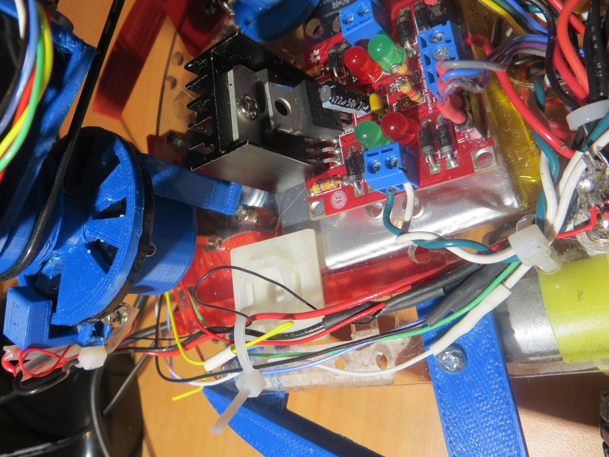
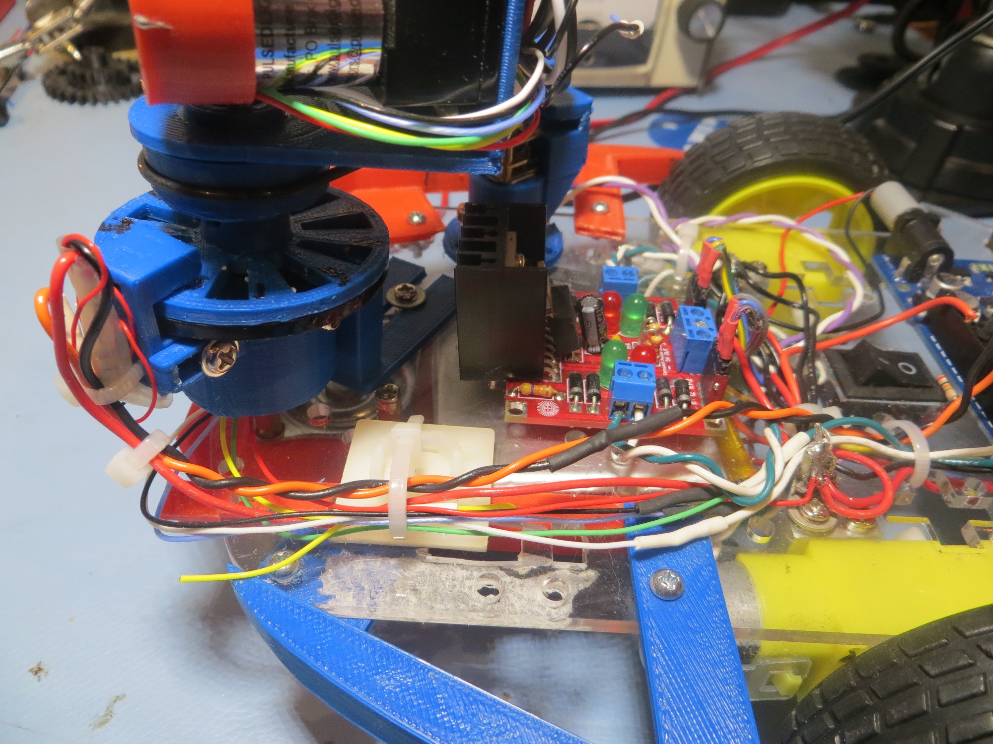
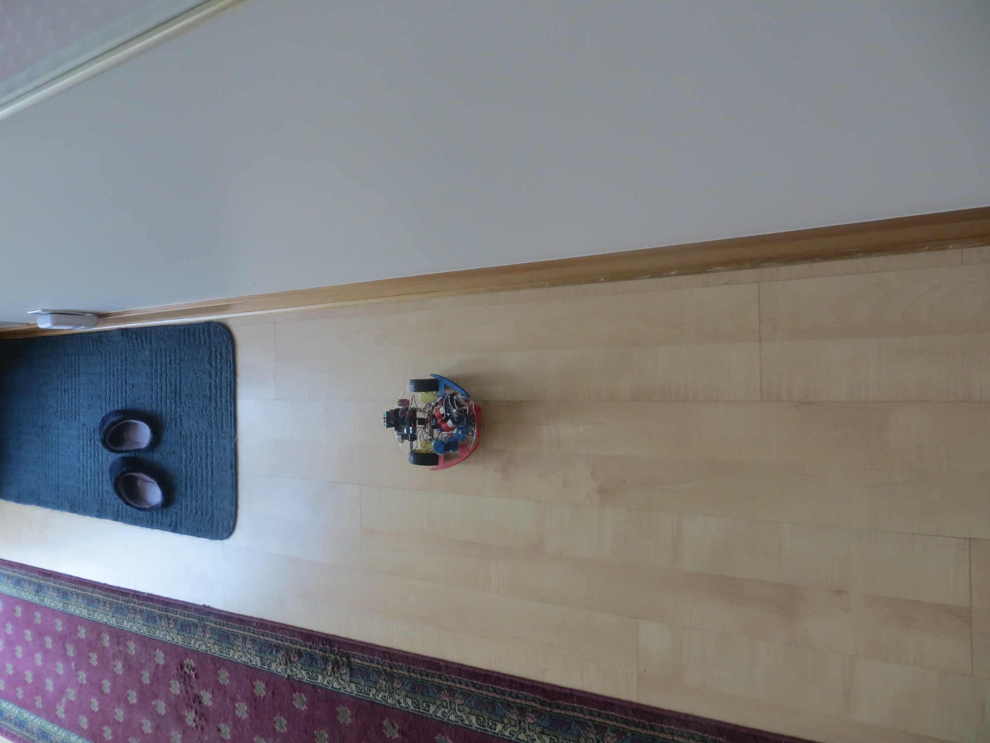
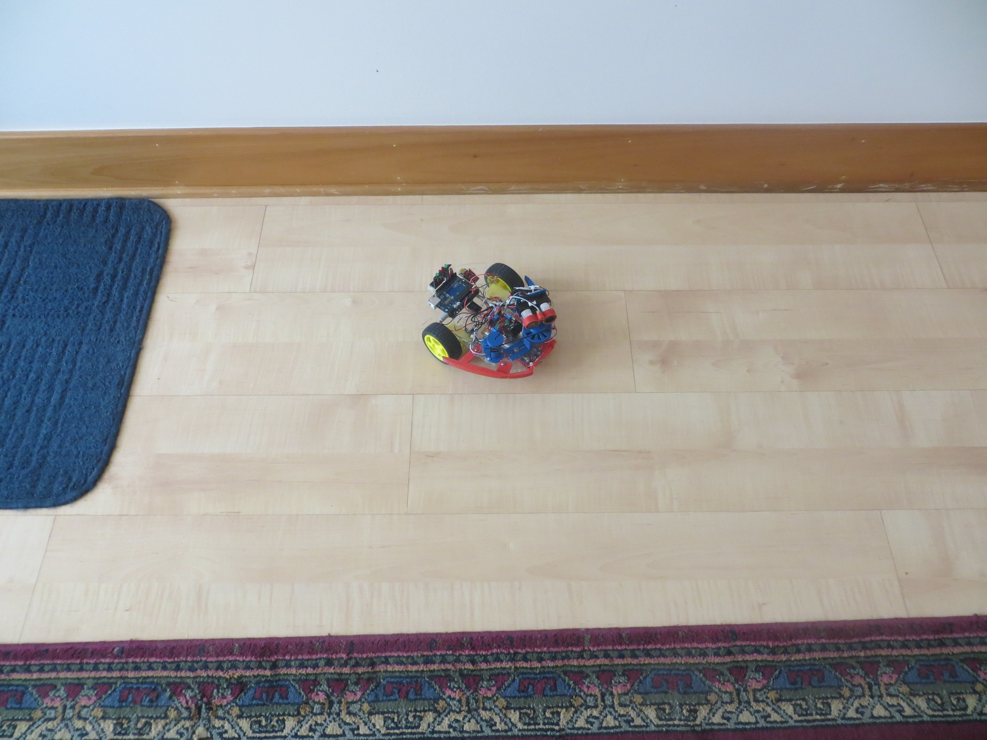
Once I had the EEPROM write/read problem solved, it was time to integrate that facility back into my LIDAR test vehicle (aka ‘Wall-E’) to see if I could capture real LIDAR data into EEPROM ‘on the fly’ using the interrupter wheel interrupt scheme I had already developed. I didn’t really need the cardboard box restriction for this, so I just set Wall-E up on my workbench and fired it up.
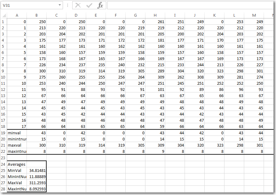
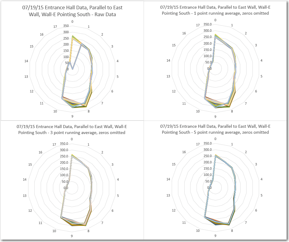
To verify proper operation, I first looked at the ‘raw’ LIDAR data coming from the spinning LIDAR setup, both in text form and via Excel’s ‘Radar’ plot. A sample of the readout from the program is shown below:
1 2 3 4 5 6 7 8 9 10 11 12 13 14 15 16 17 18 19 20 21 22 23 24 25 26 27 28 29 30 31 32 33 34 35 36 37 38 39 40 41 |
Servicing Interrupt 1 Servicing Interrupt 2 Servicing Interrupt 3 Servicing Interrupt 4 Servicing Interrupt 5 Servicing Interrupt 6 Servicing Interrupt 7 Servicing Interrupt 8 Servicing Interrupt 9 Servicing Interrupt 10 Servicing Interrupt 11 Servicing Interrupt 12 Servicing Interrupt 13 Servicing Interrupt 14 dist_cm time_ms angle_deg 458 6210 0 346 6222 20 64 6244 40 182 6257 60 239 6287 80 34 6302 100 45 6334 120 67 6345 140 55 6373 160 56 6392 180 59 6427 200 71 6444 220 107 6475 240 Servicing Interrupt 15 132 6493 260 153 6521 280 120 6091 300 54 6120 320 724 6191 340 writing DTA Array to EEPROM location 0 Servicing Interrupt 16 Servicing Interrupt 17 Servicing Interrupt 18 Servicing Interrupt 1 Servicing Interrupt 2 |
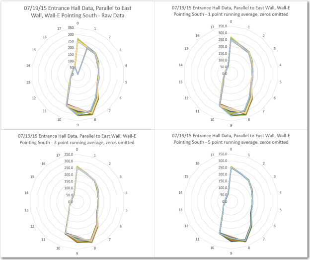
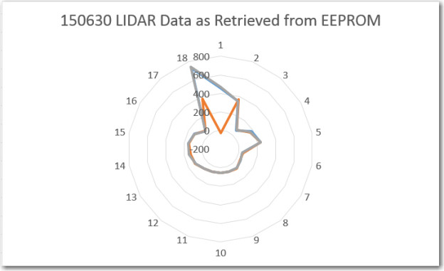
Notice the ‘Servicing Interrupt 15’ line in the middle of the (distance, time, angle) block printout. Each time the interrupt service routine (ISR) runs, it actually replaces one of the measurements already in the DTA array with a new one – in this case measurement 15. Depending on where the interrupt occurs, this can mean that some values written to EEPROM don’t match the ones printed to the console, because one or more of them got updated between the console write and the EEPROM write – oops! This actually isn’t a big deal, because the old and new measurements for a particular angle should be very similar. The ‘Radar’ plot of the data is shown below:
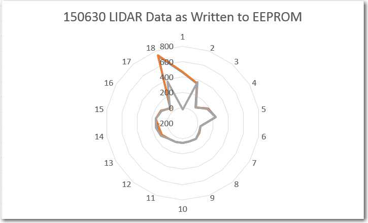
LIDAR data as written to the Arduino Uno EEPROM
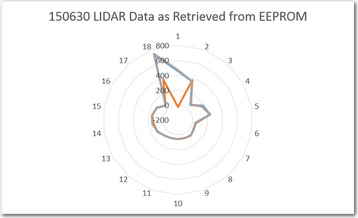
LIDAR data as read back from the Arduino Uno EEPROM
As can be seen from these two plots, the LIDAR data retrieved from the Uno’s EEPROM is almost identical to the data written out to the EEPROM during live data capture. It isn’t entirely identical, because in a few places, a measurement was updated via ISR action before the captured data was actually written to EEPROM.
Based on the above, I think it is safe to say that I can now reliably capture LIDAR data into EEPROM and get it back out again later. I’ll simply need to move the ‘readout’ code from this program into a dedicated sketch. During field runs, LIDAR data will be written to the EEPROM until it is full; later I can use the ‘readout’ sketch to retrieve the data for analysis.
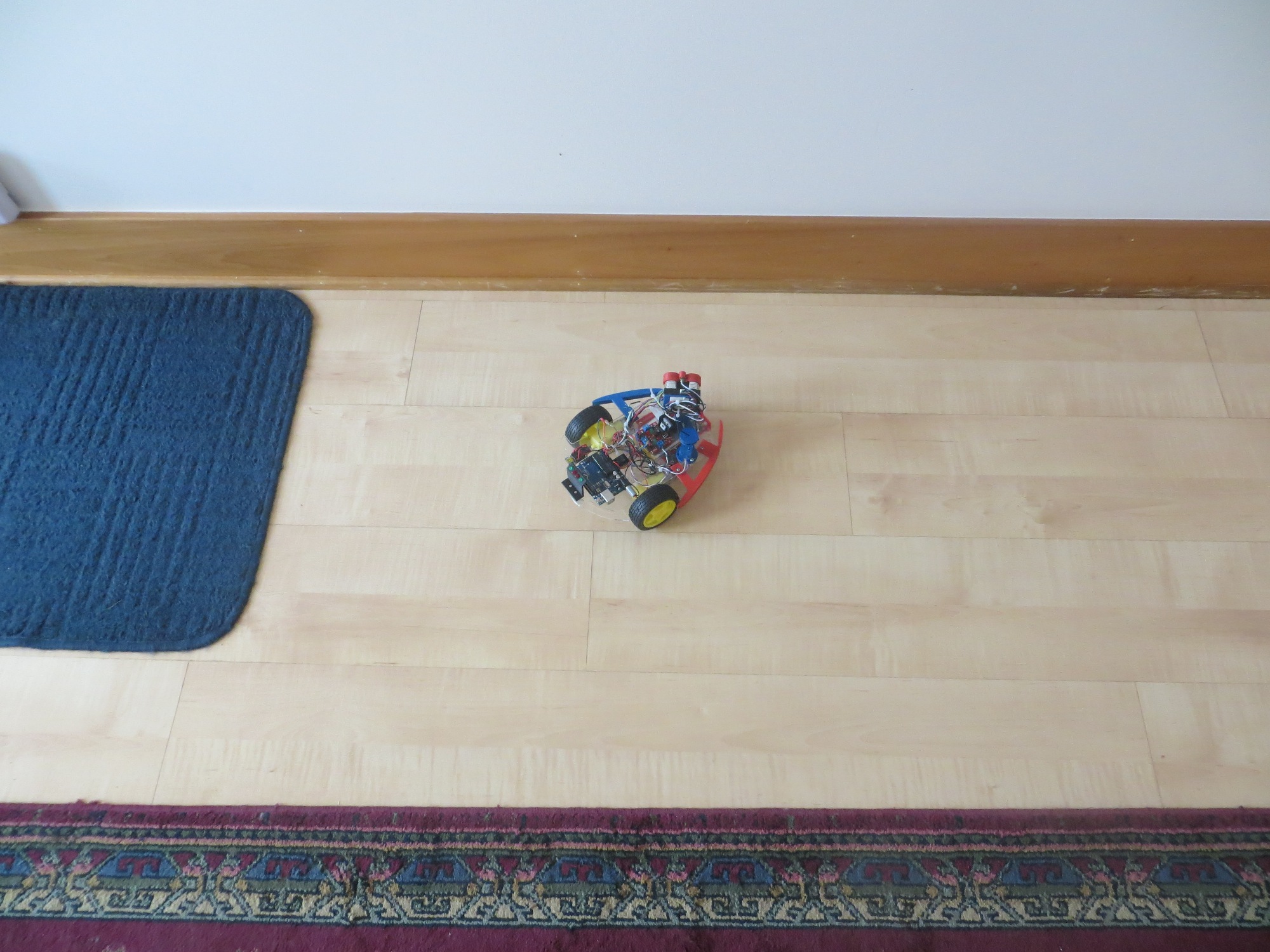
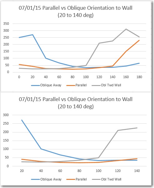
In particular, I am very interested in how the LIDAR captures a long wall near the robot. I have a theory that it will be possible to navigate along walls by looking at the relationship between just two or three LIDAR measurements as the LIDAR pointing direction sweeps along a nearby wall. Consider 3 distance measurements taken from a nearby wall, as shown in the following diagram:
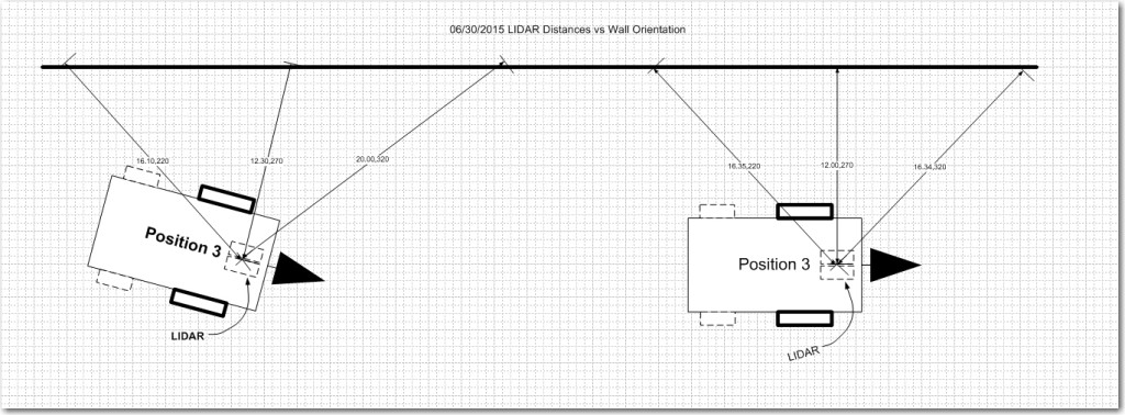
LIDAR distance measurements to a nearby long wall
In the left diagram the distances labelled ‘220’ and ‘320’ are considerably different, due to the robot’s tilted orientation relative to the nearby long wall. In the right diagram, these two distances are nearly equal. Meanwhile, the middle distance in both diagrams is nearly the same, as the robot’s orientation doesn’t significantly change its distance from the wall. So, it should be possible to navigate parallel to long wall by simply comparing the 220 degree and 320 degree (or the 040 and 140 degree) distances. If these two distances are equal or nearly so, then the robot is oriented parallel to the wall and no correction is necessary. If they are sufficiently unequal, then the appropriate wheel-speed correction is applied.
The upcoming field tests will be designed to buttress or refute the above theory – stay tuned!
Frank