Posted 6/26/2015
After getting the Pulsed Light LIDAR-Lite mounted on a spinning pedestal, and the whole thing mounted on Wall-E, it is now time to try and figure out how to use this thing to accurately map a room for navigation.
In my previous work I had developed a 10-gap (actually 9, with the 10th gap replaced by an index plug) interrupter (I no longer use the term tachometer, as it is no longer used for speed control) wheel so I could generate a rotationally-constant set of LIDAR measurement trigger signals, so I could generate 18 measurements per revolution (one for the start and end of each interrupter wheel gap. The idea was to capture these measurements (along with a computed angle and a time stamp) into an 18-element array. The array contents would be continually refreshed in real time, and then the navigation algorithm could then simply grab the latest values from the array as needed.
As always, there were a number of ‘gotcha’s’ associated with this strategy
- As currently constituted, the LIDAR is spinning at about 120 rpm – i.e. about 500 msec per rotation or about 1.4 deg/sec. Divide 500 by 18 and you get about 28 msec per interrupt time. However, a single measurement takes about 10-20 msec, which means that the distance number returned by the measurement routine isn’t where you think it is – it is rotationally skewed about 15-20 degrees – oops!
- The number returned by the measurement routine is computed by measuring the width of a pulse generated by the LIDAR that is proportional to distance. Unfortunately, this number incorporates a constant offset which must somehow be calibrated out so the result is the actual distance from some physical reference point.
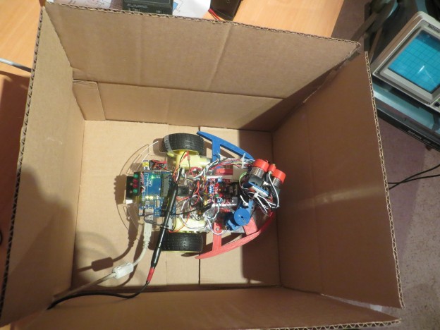
In summary, we aren’t quite sure where we are looking when we measure, and there is an unknown constant error in the distance measurements. So, how to address? The answer is the LIDAR-in-a-Box technique, as shown in the following photo.
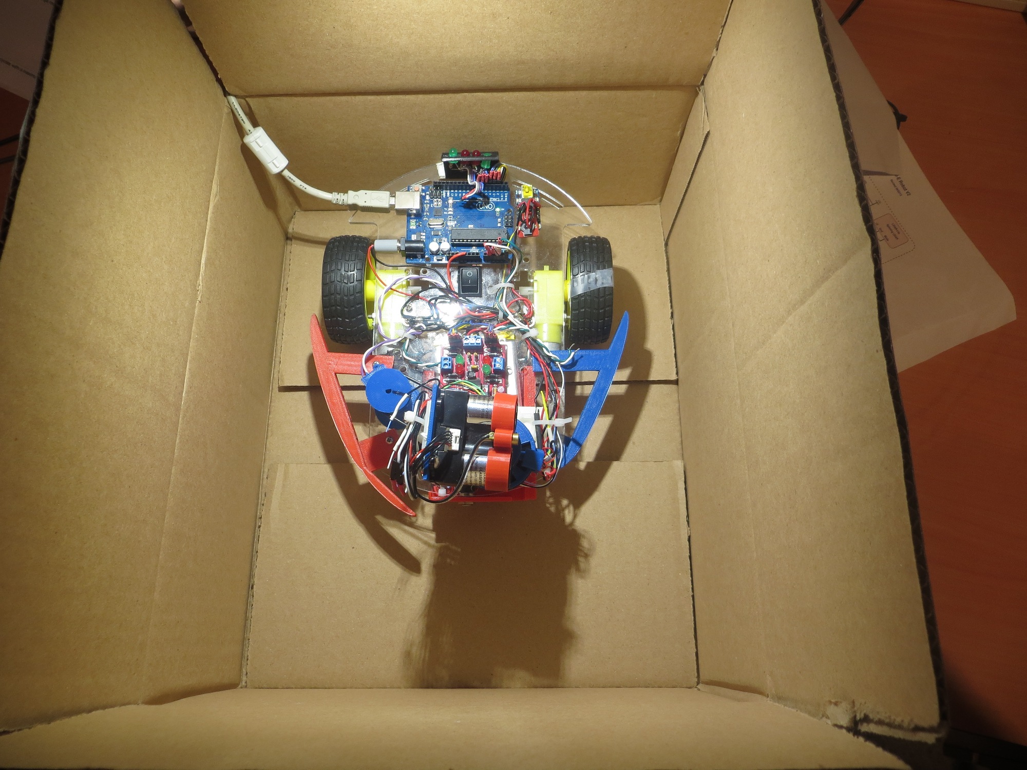
LIDAR positioned as close as possible to center of box
The idea here is to constrain the experiment to a well known geometry, which should allow both the angular and distance offsets to be determined independently of the measurements themselves. In the photo above, the LIDAR unit itself was positioned as close to the center of the box as possible, and the LIDAR line of sight was adjusted relative to the interrupter wheel such that the LIDAR unit points straight ahead when the interrupt at the trailing edge of the index plug occurs. This resulted in the following ‘radar’ plot:
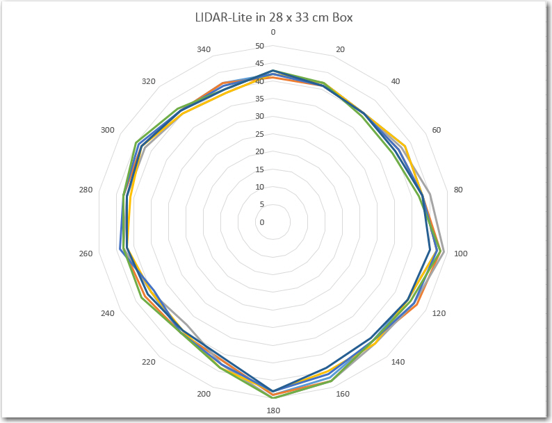
Excel ‘Radar’ plot of LIDAR Lite mounted as centrally in a 28 x 33 cm box
In the above ‘Radar’ plot, the salient points are:
- There is an offset of approximately 30 cm in all the distance measurements
- Measurements appear to be skewed angularly about 60 degrees from physical reality. I would have expected one of the two short sides to be lined up perpendicular to the 0-180 degree line, but it isn’t. Unfortunately, it is hard to tell from this plot which of the 4 sides is the ‘front’ and which are the back and/or sides.
So, I set up another experiment, with the LIDAR unit positioned as close as possible to one of the short (28 cm) sides (as shown in the following photo), and 30 cm subtracted from each measurement.
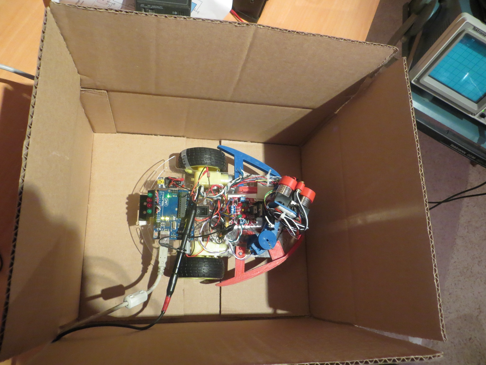
LIDAR positioned as close as possible to one end of box
The LIDAR unit relationship with the interrupter wheel was again adjusted so that it is pointed straight ahead when the index plug trailing interrupter gap starts. This was verified by triggering the co-axially mounted red laser pointer with this same interrupt, as shown in the following video (watch where the laser pointer ‘dash’ appears)
This time the Excel ‘Radar’ plot is a bit more understandable
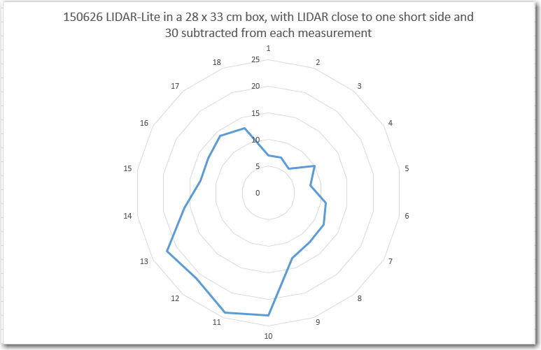
LIDAR unit positioned as close as possible to one short side
Now the plot more accurately reflects the actual box dimensions, and it is now clear which end is the ‘front’ side. Moreover, it is easy to see now that the ‘forward’ direction on the plot is skewed about 30-60 degrees from the actual physical situation. The point labelled ‘1’ on the plot should contain the value that is actually plotted opposite point ‘2’, so I suspect what is happening is that the time required for the measurement subroutine to actually return a value is on the order of one interrupt gap time after the time at which the measurement is triggered. If this is true (to be determined with future experiments), I should be able to correct for this with some ‘index gymnastics’ i.e. putting the measurement from interrupt N in the table at location N-1.
06/28/15 Update: Here’s a plot with measurements stored in the location immediately preceding the interrupter gap number. For instance, the measurement at gap 3 is stored in the 2nd dta_array location rather than the third, and so on. As can be seen, the box outline is now much better aligned with ‘straight ahead’.
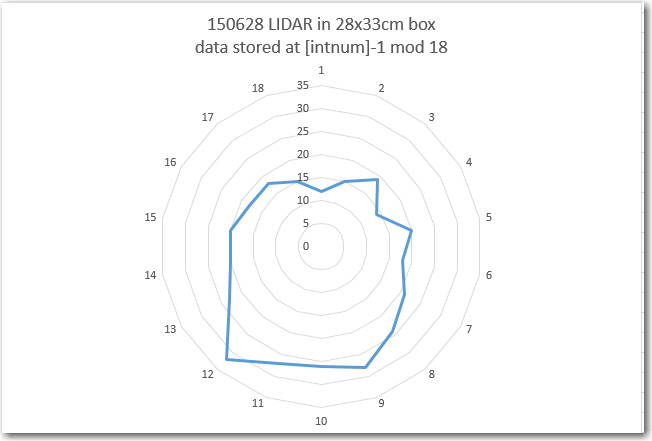
Excel ‘Radar’ plot under the same conditions as before, but with the measurement storage location shifted one location ‘down’
Stay tuned!
Frank
Pingback: Field test prep - writing to and reading from EEPROM - Paynter's Palace