Posted 04/06/15
In the last episode of the ‘stuck’ detection saga, I added a second forward-looking ping sensor above the existing one, on the theory that this would help address the ‘stealth slipper’ issue. However, field trials with the new system didn’t really show much improvement – Wall-E still gotstuck and couldn’t seem to figure it out without help.
To try and clarify what was going on, I disabled the normal forward obstacle avoidance maneuver that is triggered whenever Wall-E gets within about 10cm of an object. This caused the robot to run right into forward obstacles without stopping. The idea was to see if the ‘stuck’ detection algorithm would take over and get Wall-E free. As it turned out, the robot would simply sit there forever with its nose pushed firmly up against whatever it was stuck on.
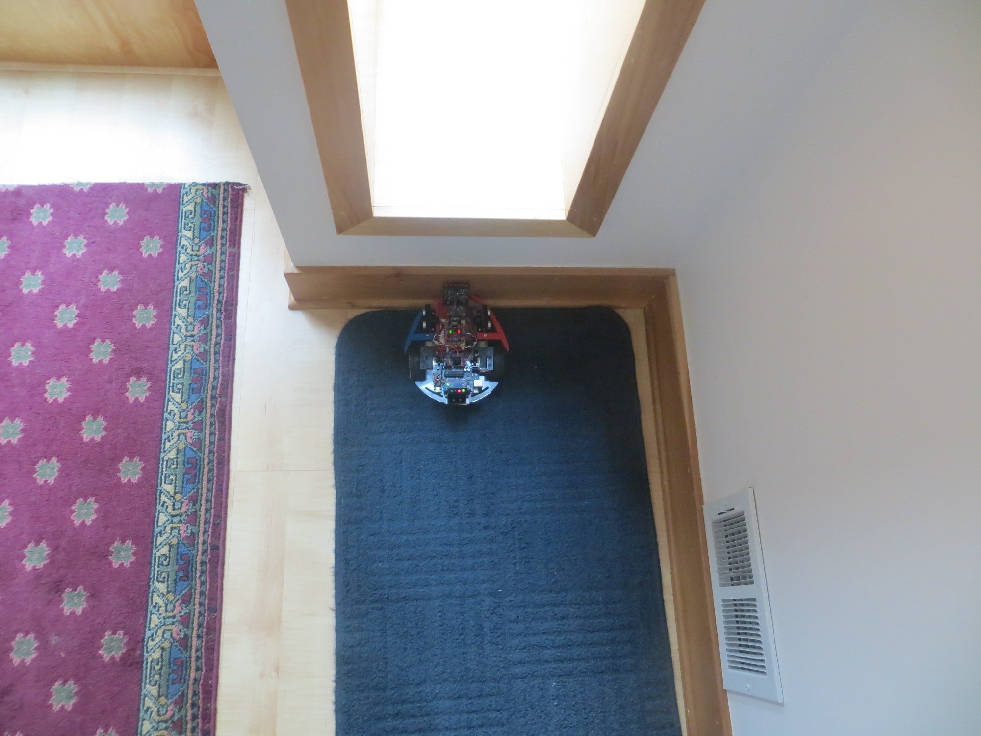
Classic Wall-E ‘Nose Plant’ position
The ‘stuck’ detection algorithm was designed to trigger when the variation in distance readings from the left, right, and top-forward sensors falls below a settable threshold, as should be true whenever Wall-E gets stuck. In the field trials, this seemed to be exactly what was happening, except Wall-E never figured it out. After scratching my head about this for a while, I noticed that I could sometimes trigger Wall-E’s ‘stuck’ detection routine by placing a foot in the field of view of one of the side sensors, typically the one on the opposite side from the nearest wall, as shown below.
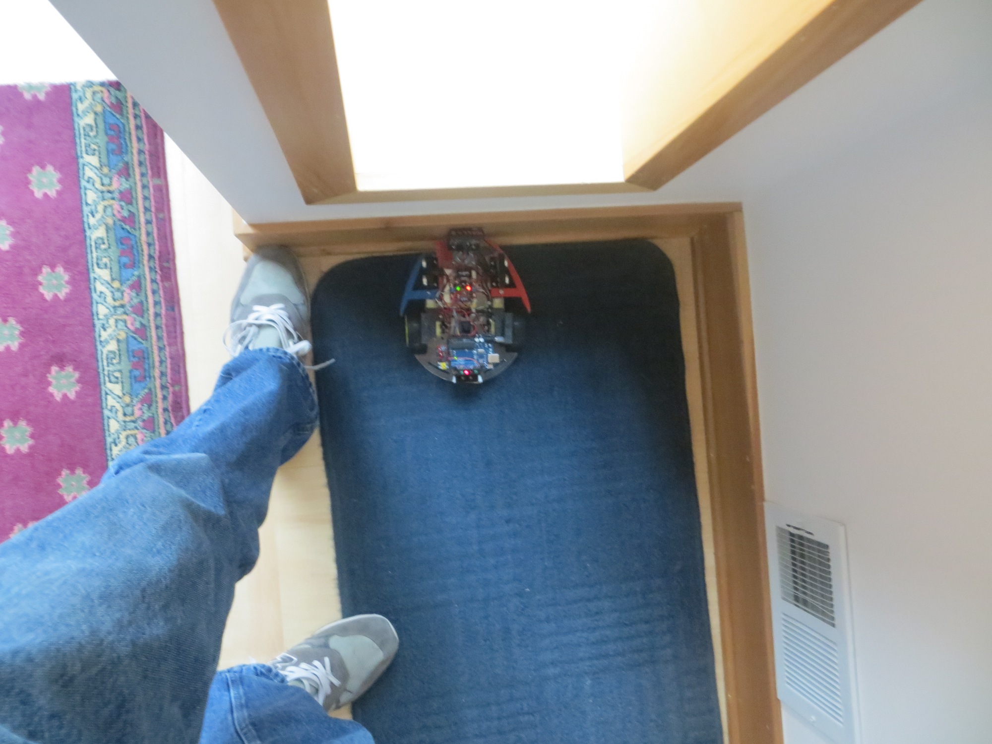
This sometimes triggered the ‘stuck’ detection routine
This technique wasn’t terribly consistent, but it did work enough times to make me think that I was on to something. I began to think that the ‘offside’ sensor distance readings contain sufficient variability to defeat the ‘stuck’ detection algorithm, even though the geometry is completely static, and the sensors are supposed to report 0 if the nearest obstacle is beyond the preset distance limit (200 cm in my case).
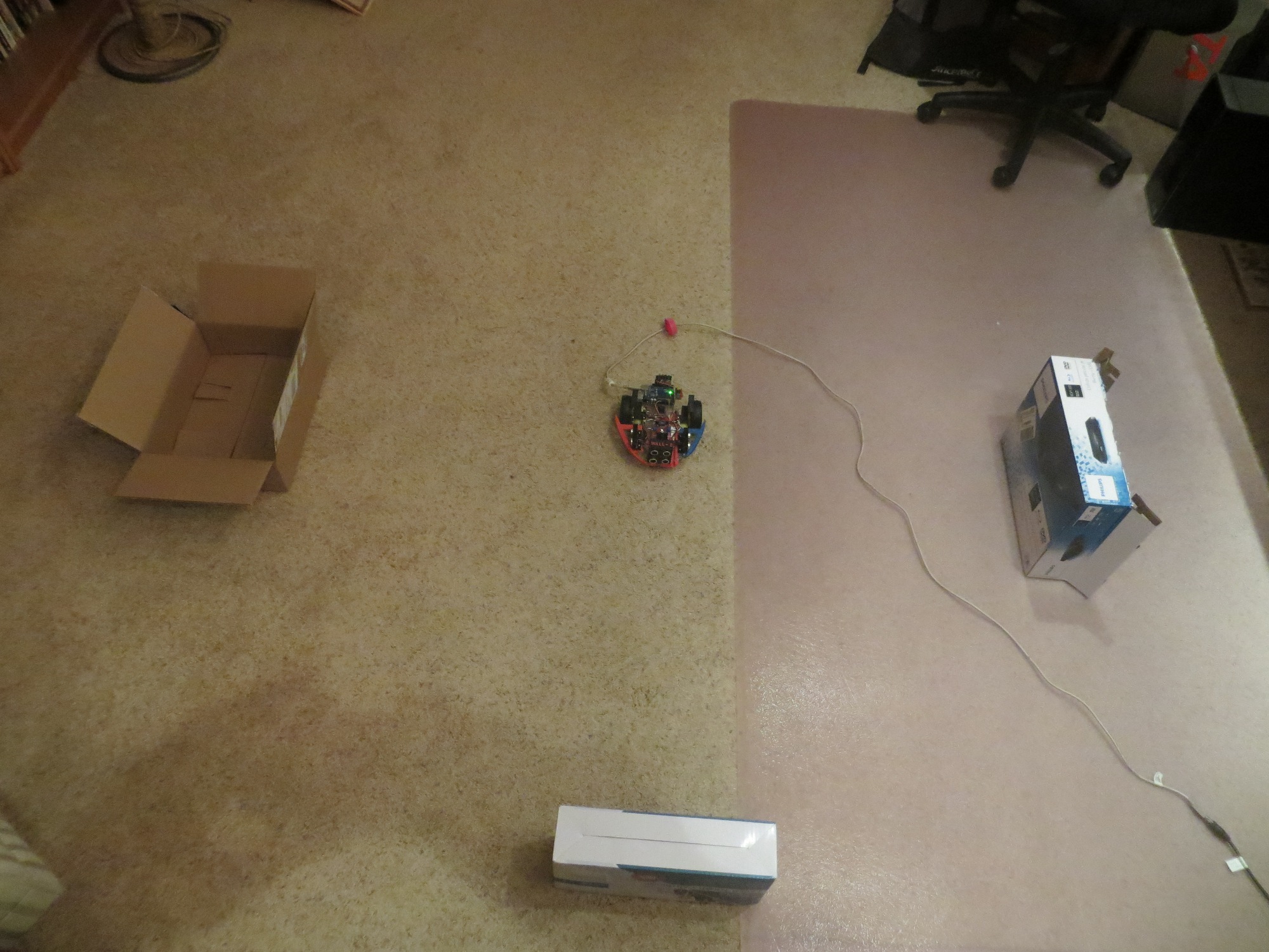
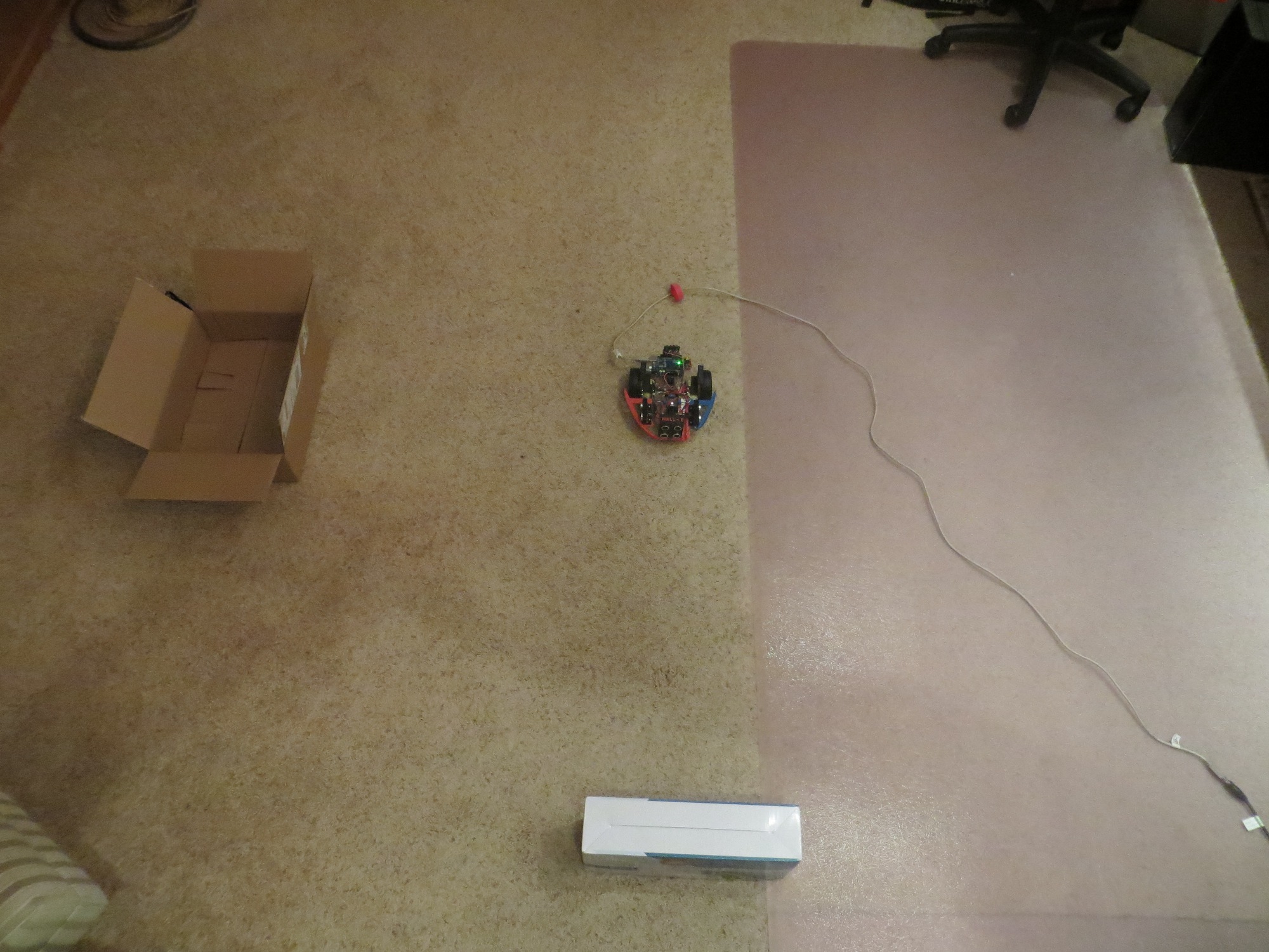
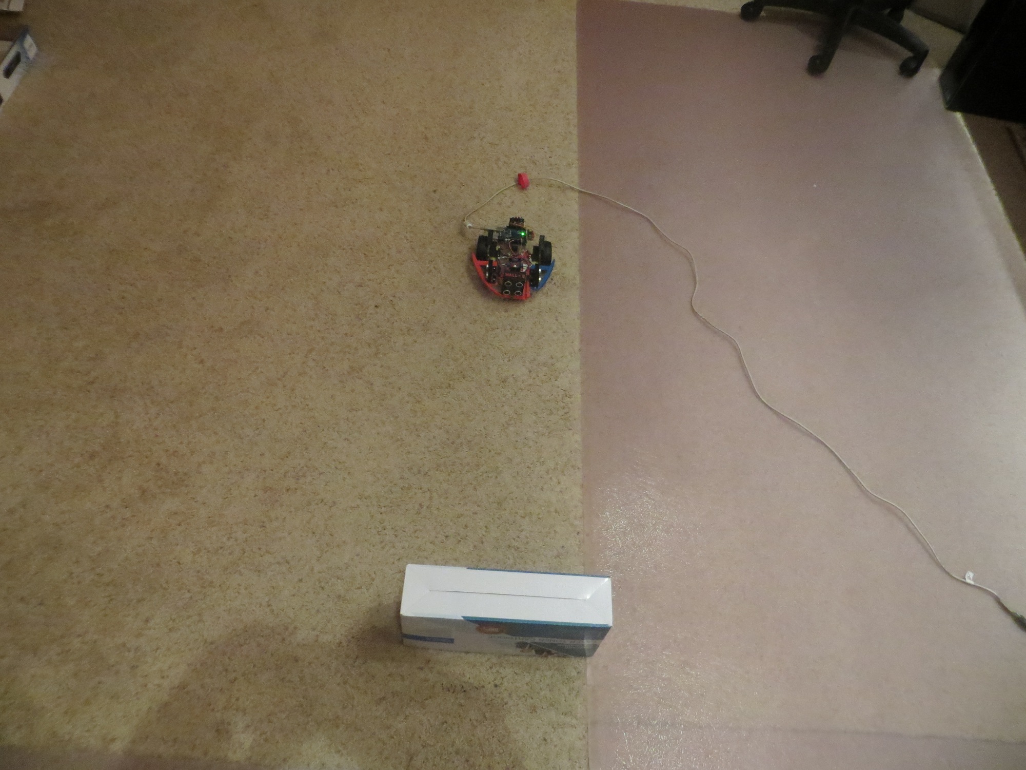
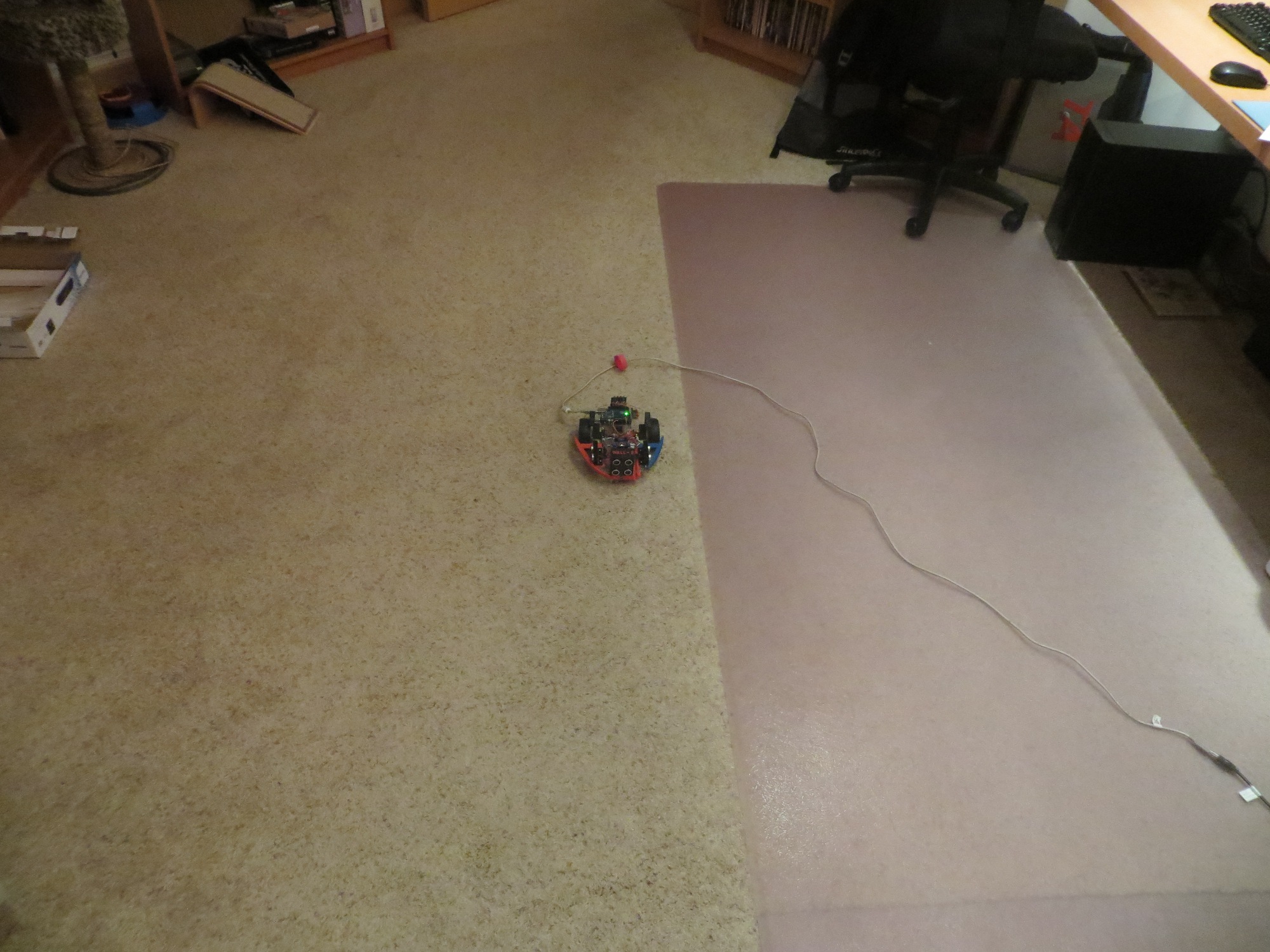
After trying various combinations in the field trials, I decided to try to set up a more rigorous testing environment. So, I connected Wall-E to my PC using a longish USB cable and set him on the floor of my lab, in a position where all four ping sensors were clear of obstacles for at least 200 cm. The use of the USB cable also allowed me to power the Arduino without powering the motors, thereby eliminating a set of variables. Then I placed an acoustically solid obstacle at various distances away from the front sensor and watched what happened.
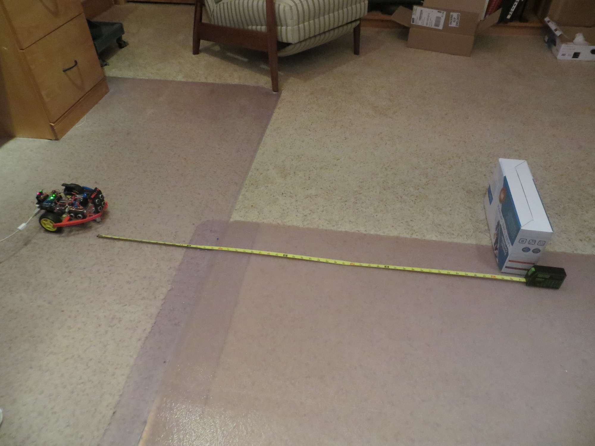
The Wall-E Indoor Acoustic Sensor Test Range
What I discovered was that Wall-E, when left alone with nothing in range of any ping sensor, will never declare itself stuck, even when it is clearly sitting still (motor drives disabled)! However, if there is an object within range of any sensor, then it will shortly detect the ‘stuck’ condition.
The clear implication of this observation is that the sensor response with nothing in view is not constant, but has sufficient variation to overwhelm the ‘stuck’ detection algorithm. This appears to be contrary to the NewPing library specification, which states that the response to a ping where there is no object within the specified max detection range will be constant (zero, actually). OTOH it is possible that my current 200 cm max range specification is too large, and what is happening is intermittent detection of objects that are nearly 200 cm away, and sometimes a zero is returned and sometimes not.
The only direct way to clear up the mystery is to look at the actual ping sensor data in the ‘no object in view’ case and see what is returned. To do this I will probably need to create a specialized Arduino program to take the data and then report it.
So, I created a new Arduino sketch called ‘PingTest1’ (clever name, huh?) that simply reports the contents of the left, right, and top-front ping sensor arrays about once per second. This data was then sucked into Excel and graphed. Four different physical configurations were tested, in the following order:
- Obstacles at about 75 cm in view of all three sensors (Figure 1)
- Left obstacle removed (Figure 2)
- Left and right obstacles removed (Figure 3)
- All three obstacles removed (Figure 4)
Obstacles at about 75 cm From Left, Right, and Front Sensors
Left Obstacle Removed
Left and Right Obstacles Removed
All 3 Obstacles Removed
This produced the overall plot shown below. The first 200 or so data points show the process of replacing the initial zero state of the distance arrays with real values as they are acquired. The left obstacle is removed at about item 1000, the right obstacle at about item 1700, and the front one at about 2800.
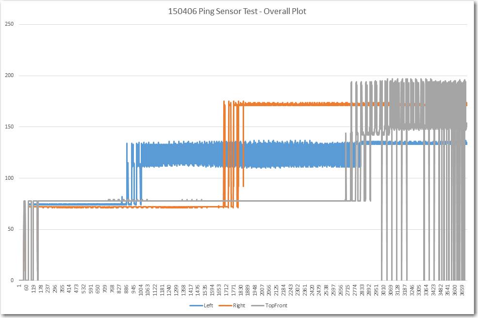
Overall plot of approximately 3600 sets of sensor readings
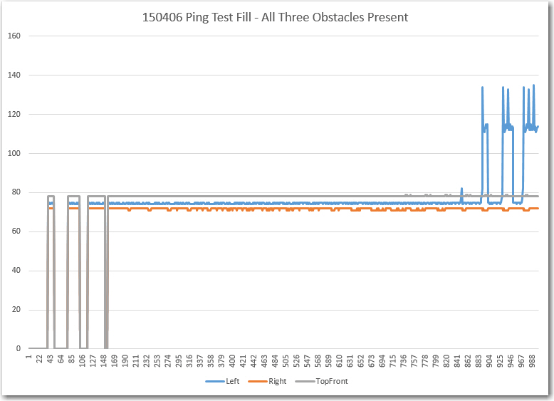
First 1000 or so points, showing the fill procedure and the response with all 3 obstacles present
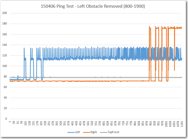
From about 800 to 1900, showing the responses with the left obstacle removed
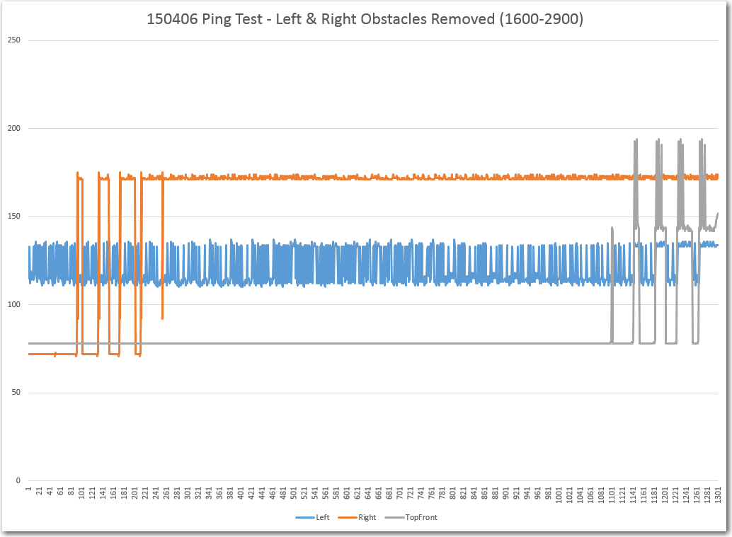
From 1600 or so to 2900, showing the Left and Right obstacles removed
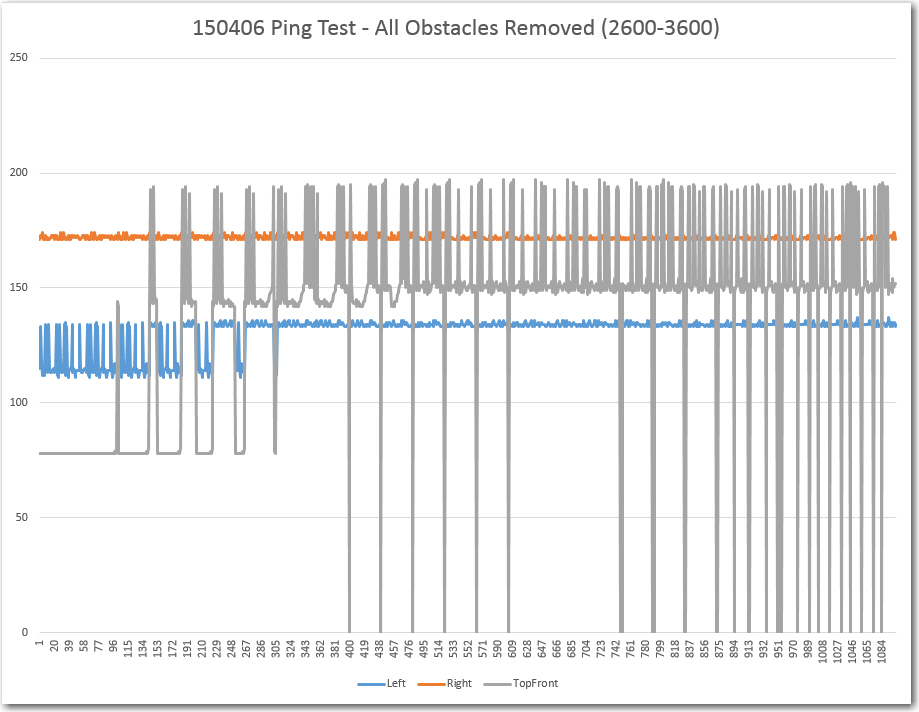
From about 2600 to 3600, showing the responses with all 3 obstacles removed. Note the large variations returned by the top front ping sensor
My general impression after looking at this data was “What a mess!”. I’ll never be able to detect a ‘stuck’ condition with all this variation, especially the HUGE (over 50 cm) high-frequency variation in the top front distance readings, not to mention the less frequent (but no less disastrous) rail-to-rail excursions from nearly 200 to 0 and back again. However, there are some features about this data that make me think I’m not completely out of luck. The response with all three obstacles present is quite clean – with less than 2 cm variation on all three channels. I believe this section explains why I was occasionally able to get Wall-E to detect the ‘stuck’ condition if I placed an obstacle (my foot) in view of whichever side sensor was ‘staring off into space’. It also explains why I had to use both feet when both the left and right sensors had no nearby wall features in view. By inserting an obstacle into the sensors’ view, I was moving the configuration from the right side of the overall plot above, with all its ugly variation, to the left side where the data is nice and clean with very little variation over time.
However, I’m at a complete loss to explain the large variation in the left sensor distance measurements with the left obstacle removed. I can rationalize the mean number of about 120 cm as coming from items under my work surface on the left side, but all that stuff is static – no movement at all! When the right obstacle is removed, it’s readings jump from about 75 to about 175 cm, consistent with the distance to my bookcase on that side, and the readings continue to be quite clean – less than 4 cm variation across the entire period. Then there is the double (or is it triple) mystery of what happens when the front obstacle is removed. The front distance reading goes from about 75 to about the same average as the right sensor, but the variation is HUGE – 50 cm or more! And just to add to the mystery pile, the variations in the left sensor distance readings largely disappear – how can that possibly happen? It actually looks like there is some relationship between the removal of the front obstacle and the disappearance of the variation from left sensor readings – how can that be? Is there some external feedback between the front and left sensors that isn’t present between the front and right sensors? Could the ping timing be such that a ping is emitted from the front sensor, bounces off the front obstacle and then some objects in the field of view of the left sensor, arriving at the left sensor just in time to look like a valid echo? I think I’m getting a headache! ;-).
Although this data raised as many questions as it answered, it is definitely a step in the right direction. Now I need to repeat this experiment with some modifications, as follows:
- Do the same experiment with the front ping sensors disabled, to eliminate the possibility of echo contamination between the front and left and/or right sensors.
- Look at the front ping sensor response when Wall-E’s nose is pressed up against a wall. This won’t normally be an issue, as Wall-E’s normal obstacle avoidance routine will make it stop and turn around when it gets within about 10 cm of an obstacle, but I have disabled that while trying to work out the ‘stuck’ detection issues. So, I need to understand just what is happening in this case.
- Change the MAX_DISTANCE_CM parameter from 200 to 100. It is clear to me from my lab ‘indoor test range’ experiments that 100 cm in each direction is more than enough to handle almost all situations in my house, and if this change eliminates the wild variations with no object in view, so much the better.
More to come,
Frank